
Euler Equations for Outer Flow
Enroll to start learning
You’ve not yet enrolled in this course. Please enroll for free to listen to audio lessons, classroom podcasts and take practice test.
Interactive Audio Lesson
Listen to a student-teacher conversation explaining the topic in a relatable way.
Introduction to Boundary Layers
🔒 Unlock Audio Lesson
Sign up and enroll to listen to this audio lesson

Today we are going to discuss boundary layers. Can anyone tell me what a boundary layer is?

Isn’t it the thin layer of fluid that forms near a solid surface when a fluid flows past it?
Exactly! The boundary layer is crucial because it determines how the fluid interacts with the surface. Can anyone guess why it's important?

It affects the drag force on the object, right?
That’s right! We often analyze these effects to improve designs in fields such as aerospace. Now, let’s remember this concept with the acronym B.L.A.C. – Boundary Layer Affects Drag Calculations.

So, if we understand boundary layers, we can optimize drag?
Precisely! Understanding how these layers behave helps in design efficiency. Great start! Let’s dive deeper into how these layers are characterized.
Reynolds Numbers and Flow Types
🔒 Unlock Audio Lesson
Sign up and enroll to listen to this audio lesson

Continuing from our discussion, who can explain the significance of Reynolds numbers in flow behavior?

Reynolds numbers help us determine whether the flow is laminar or turbulent.
Correct! When the Reynolds number is less than 10^5, the flow is typically laminar. What about when it's greater?
Then it becomes turbulent, right?
That's right! To remember this crucial point, think of the rhyme: 'Under fifty thousand, we flow like a stream, over three million, we’re turbulent it seems!'
That’s a catchy way to remember it! How do we experimentally validate these numbers?
Good question! We perform experiments in wind tunnels to measure and analyze how flow behaves under different conditions. Let’s move on to how we derive equations for these boundary layers.
Derivation of Boundary Layer Equations
🔒 Unlock Audio Lesson
Sign up and enroll to listen to this audio lesson
Now, let’s discuss how we derive boundary layer equations. Can anyone recall the primary equations we start with?
Are we starting with the Navier-Stokes equations?
Yes! We use the Navier-Stokes equations and simplify them, negating terms that are not significant for the boundary layer. What do we negate?
Gravity forces and local acceleration terms?
Exactly! This leads us to the boundary layer equations. To help memorize the steps, think of the acronym G.L.A. – Gravity Left And Acceleration Neglected.
What do we obtain with these simplifications?
We derive equations that are easier to solve, especially with modern computational methods. Let’s proceed to tackle more about the assumptions underlying these equations.
Applications in Engineering
🔒 Unlock Audio Lesson
Sign up and enroll to listen to this audio lesson
Finally, let’s reflect on the application of the knowledge gained about boundary layers in engineering fields. How do they help us?
They help in optimizing designs to minimize drag!
Correct! By predicting boundary layer behavior, we can enhance system designs across different industries. What might be a real-world example?
In aerospace engineering, we need boundary layer control for airplane wings to reduce drag and improve fuel efficiency.
Great example! Remember the acronym A.D.D. – Application Drives Design. This encapsulates the importance of our topic today.
How can computational tools help with boundary layer analysis?
Computational fluid dynamics (CFD) tools allow us to simulate and analyze fluid flows in ways that were not possible before. Well done today, everyone!
Introduction & Overview
Read summaries of the section's main ideas at different levels of detail.
Quick Overview
Standard
The section provides a detailed examination of boundary layers in fluid dynamics, including the derivation of boundary layer equations and their application in analyzing flow over surfaces like flat plates. Discussion on laminar and turbulent flows, as well as experimental observations related to Reynolds numbers, is included.
Detailed
In fluid mechanics, the boundary layer concept is pivotal for understanding how fluids behave as they interact with solid surfaces. This section provides an insight into boundary layer approximations, particularly focusing on the simplifications made when analyzing flow using Euler equations and Navier-Stokes equations. The section begins by introducing boundary layers and illustrating their effects through laminar flow in simple geometries.
A foundational element discussed is the no-slip boundary condition, set against the backdrop of Reynolds numbers which determine flow characteristics. When the Reynolds number is below 10^5, the flow remains laminar, transitioning to turbulence as it exceeds approximately 3x10^6. Experimental validations from wind tunnels are highlighted, demonstrating how these concepts are necessary for applications in engineering contexts, such as automotive and aerospace design.
In the explanation, the derivation of boundary layer equations from Navier-Stokes equations is summarized, including assumptions that simplify the equations under certain conditions, such as neglecting gravity forces due to their minimal impact compared to inertial forces. It wraps up by emphasizing the solutions to these equations through modern computational fluid dynamics (CFD) tools, illustrating the evolution from analytical methods to numerical approaches in solving fluid flow problems.
Youtube Videos

![Euler's Equation Concept [Fluid Mechanics]](https://img.youtube.com/vi/-wI3PpWc7L8/mqdefault.jpg)


Audio Book
Dive deep into the subject with an immersive audiobook experience.
Introduction to Boundary Layer Concept
Chapter 1 of 5
🔒 Unlock Audio Chapter
Sign up and enroll to access the full audio experience
Chapter Content
Understanding the utility of boundary layers is crucial as they appear in various flow scenarios, such as mixing layers, wake formations, and jet formations. The boundary layer equations are derived from approximations of the Navier-Stokes equations.
Detailed Explanation
Boundary layers are thin regions at the surface of an object where effects of viscosity are significant, impacting how fluid flows over surfaces. They are vital for understanding fluid mechanics, especially in applications like aerodynamics and hydrodynamics. Basic flow cases often involve boundary layers that can be approximated using simpler equations derived from the complex Navier-Stokes equations, which describe fluid motion in detail. These approximations simplify the analysis, making it feasible to predict flow behavior such as drag and lift in engineering applications.
Examples & Analogies
Imagine a boat moving through water. When the boat moves, water flows around it – the layer of water closest to the boat's hull (where the water moves slower due to friction) is similar to a boundary layer. Understanding how this layer behaves helps in designing the boat’s shape for reduced drag, just like how car manufacturers study airflow around vehicles.
Key Assumptions in Boundary Layer Equations
Chapter 2 of 5
🔒 Unlock Audio Chapter
Sign up and enroll to access the full audio experience
Chapter Content
Boundary layer approximations make several assumptions, such as steady flow, two-dimensional flow, and neglecting gravity force. The primary focus remains on the viscous forces in the boundary layer.
Detailed Explanation
When applying boundary layer theory, several critical assumptions are made. The flow is assumed to be steady (not changing with time), and largely two-dimensional (varying in the x and y directions but not significantly in the z direction). Gravity forces are typically negligible compared to inertial forces in a horizontal flow situation. These assumptions facilitate the derivation of simpler equations that can effectively predict the behavior of the fluid in the boundary layer while focusing on the viscous effects that dominate near the surface.
Examples & Analogies
Think about how air flows over airplane wings. Designers assume steady airflow to simplify calculations, just as they assume a two-dimensional flow to make complex aerodynamics more manageable. By simplifying these aspects, engineers can focus on the critical factors affecting flight performance, such as lift and drag.
Characteristics of Laminar and Turbulent Flow
Chapter 3 of 5
🔒 Unlock Audio Chapter
Sign up and enroll to access the full audio experience
Chapter Content
The transition of flow behavior is notable depending on the Reynolds number. Laminar flow occurs at lower Reynolds numbers, while turbulent flow arises when Reynolds numbers exceed certain values.
Detailed Explanation
The Reynolds number helps categorize flow regimes. Laminar flow, characterized by smooth and orderly motion, occurs when the Reynolds number is below 100,000. When the Reynolds number exceeds around 3,000,000, flow becomes turbulent, which is chaotic with eddies and fluctuations. Understanding these transitions is crucial for predicting the flow's behavior and designing efficient systems, such as pipelines and aircraft.
Examples & Analogies
Consider a river flowing gently: the water moves smoothly in layers — that's laminar flow. Now, imagine a storm that increases the river's flow rate: the water becomes choppy and unpredictable — this is akin to turbulent flow. Engineers must understand these behaviors to design structures that can handle both calm and stormy conditions.
Deriving the Boundary Layer Equations
Chapter 4 of 5
🔒 Unlock Audio Chapter
Sign up and enroll to access the full audio experience
Chapter Content
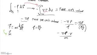
The derivation of boundary layer equations involves applying order-of-magnitude analysis to the Navier-Stokes equations. By assuming certain velocity relationships and vectors, we rewrite the equations to focus on relevant quantities.
Detailed Explanation
To derive the boundary layer equations, we start with the Navier-Stokes equations, which govern fluid motion. By applying order-of-magnitude analysis, we can simplify these equations by identifying which terms are significant and which can be neglected. This analysis leads to two central equations: one for continuity and another that incorporates viscous effects, allowing us to analyze flow in boundary layers effectively.
Examples & Analogies
Think of a traffic flow at a busy intersection. At peak times, analyzing every vehicle’s speed (like every term in the Navier-Stokes equations) can be overwhelming. Instead, traffic engineers focus on key factors impacting congestion (critical terms), allowing them to design better traffic signals and road layouts — analogous to how we derive boundary layer equations by focusing on the most influential factors.
Numerical Solutions and Practical Application
Chapter 5 of 5
🔒 Unlock Audio Chapter
Sign up and enroll to access the full audio experience
Chapter Content
Modern computational fluid dynamics (CFD) techniques allow solving boundary layer equations efficiently, providing valuable insights into velocity distributions and pressure variations along surfaces.
Detailed Explanation
With advancements in technology, numerical methods enable quick and accurate solutions to the boundary layer equations. These numerical simulations can help predict how fluid behaves around objects, aiding in the design of various engineering systems such as aircraft, cars, and buildings by understanding forces acting on them.
Examples & Analogies
Imagine using a weather app that predicts rain. This app uses complex models to simulate atmospheric conditions, much like CFD does for fluid flow. By inputting specific parameters, just as we do with airflow conditions, these numerical tools can forecast potential problems and help design better systems, just like how understanding weather patterns helps us prepare for storms.
Key Concepts
-
Boundary Layer: The thin fluid layer that forms near solid surfaces affecting flow behavior.
-
Reynolds Number: A critical parameter that determines if flow is laminar or turbulent.
-
Navier-Stokes Equations: Fundamental equations describing fluid dynamics adjusted for boundary layer calculations.
-
Euler Equations: Governing equations for inviscid flows, which can be used for approximating boundary layer influences.
Examples & Applications
The behavior of air flowing over an aircraft wing, where the boundary layer affects lift and drag.
Simplified experiments in wind tunnels to measure how different Reynolds numbers affect flow over flat plates.
Memory Aids
Interactive tools to help you remember key concepts
Rhymes
When Reynolds is up high, turbulence runs wild, but when it’s low, smooth flow's compiled.
Stories
Imagine a serene river flowing gently past a rocky bank. This represents laminar flow, but when the wind stirs up waves, we see turbulent flow.
Memory Tools
Remember B.L.A.C: Boundary Layer Affects Drag Calculations.
Acronyms
G.L.A
Gravity Left And Acceleration Neglected
emphasizes simplifications in boundary layer derivations.
Flash Cards
Glossary
- Boundary Layer
A thin layer of fluid near the surface of a solid object where the effects of viscosity are significant.
- Reynolds Number
A dimensionless number used to predict flow patterns in different fluid flow situations.
- NavierStokes Equations
Mathematical equations that describe the motion of viscous fluid substances.
- Euler Equations
Equations that describe the motion of inviscid flow (flows with negligible viscosity).
- Laminar Flow
A flow regime characterized by smooth, predictable fluid motion, typically occurring at low Reynolds numbers.
- Turbulent Flow
A flow regime characterized by chaotic and irregular fluid motion, usually occurring at high Reynolds numbers.
Reference links
Supplementary resources to enhance your learning experience.