
General Characteristics of DAD Curves
Enroll to start learning
You’ve not yet enrolled in this course. Please enroll for free to listen to audio lessons, classroom podcasts and take practice test.
Interactive Audio Lesson
Listen to a student-teacher conversation explaining the topic in a relatable way.
Relationship Between Rainfall Depth and Area
🔒 Unlock Audio Lesson
Sign up and enroll to listen to this audio lesson

Today, we'll discuss how the depth of rainfall changes based on the area it covers. Can anyone tell me what happens to rainfall depth as our focus area increases?

It probably decreases since the same amount of rain is spread over a larger area.
That's right! When the area increases, the average depth tends to decrease. We can remember this with the acronym 'DAMP' - Decreasing Average with More Precipitation. Let's explore how this works.

So, is there a specific ratio we can use or just a general trend?
It’s more of a trend, but we can use historical data to build DAD curves that reflect these relationships accurately. Does anyone know why it’s important to understand this relationship?

It helps in flood planning and predicting rainfall's effect on different environments right?
Exactly! Understanding these relationships is crucial for hydrologic design and flood estimation!
Impact of Duration on Rainfall Depth
🔒 Unlock Audio Lesson
Sign up and enroll to listen to this audio lesson

Now, let’s look at how rainfall depth behaves when the storm duration changes but the area stays the same. What do you think happens?

I think it would increase, since a longer storm should allow more rain to fall.
Correct! Depth increases with duration up to a limit. We remember this with 'LID' - Length increases Depth. Can anyone explain why there's a limit?
Maybe there's a point where the area’s saturation prevents more rainfall from being beneficial?
Great observation! Once saturation occurs, additional rainfall doesn't increase depth meaningfully. This helps us in flood modeling. Why do you think this understanding matters in engineering?
It's vital for designing infrastructure that can handle potential flooding.
Exactly! Engineers rely on these insights to create resilient systems.
Curve Behavior and Flattening
🔒 Unlock Audio Lesson
Sign up and enroll to listen to this audio lesson
Finally, let's talk about the behavior of DAD curves for large areas or durations. What happens to these curves as we analyze bigger data sets?
They must flatten out because the average gets diluted over a broader area or longer time, right?
Exactly! This phenomenon is due to spatial and temporal averaging. Can you see how this could influence flood analysis?
Yes! A flatter curve means that extreme rainfall events are less localized.
Well put! Remember this when considering design limits and flood mitigation strategies. Why do you think it’s necessary to plot these curves on specific scales, like log-log?
I think it’s to better visualize the relationships as they can span wide ranges of values.
Exactly! Using log scales gives us a clearer perspective on such relationships.
Introduction & Overview
Read summaries of the section's main ideas at different levels of detail.
Quick Overview
Standard
DAD curves depict how rainfall depth decreases with increasing area for a fixed duration, and vice versa. They are critical for understanding hydrologic designs and methodologies by visualizing the interactions between precipitation characteristics.
Detailed
Detailed Summary of General Characteristics of DAD Curves
The General Characteristics of Depth-Area-Duration (DAD) curves focus on illustrating significant trends in the relationship between rainfall depth, the area affected, and storm duration. These essential characteristics include:
- Rainfall Depth and Area: For a fixed duration, as the area increases, the depth of rainfall generally decreases. This behavior can be attributed to the distribution of precipitation over a larger area, diluting the depth measurement.
- Rainfall Depth with Duration: Conversely, for a fixed area, the depth of rainfall tends to increase with the duration of the storm up to a specific limit, indicating that longer storms produce more accumulated precipitation.
- Curve Flattening: DAD curves exhibit a tendency to flatten out as areas or durations increase due to spatial and temporal averaging effects, reflecting how extreme heavy precipitation becomes less concentrated over larger areas.
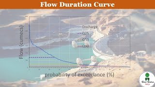
Visualization of DAD curves is typically done on a log-log or semi-logarithmic scale, with area plotted on the x-axis and rainfall depth on the y-axis, providing a useful analytical tool in hydrologic studies, including design storms and flood estimation.
Youtube Videos


Audio Book
Dive deep into the subject with an immersive audiobook experience.
Rainfall Depth vs Area
Chapter 1 of 4
🔒 Unlock Audio Chapter
Sign up and enroll to access the full audio experience
Chapter Content
• For a fixed duration, rainfall depth decreases as the area increases.
Detailed Explanation
This characteristic indicates that as the area over which rain falls gets larger, the average depth of rainfall for a specific duration decreases. For example, if you have a small garden and it receives a rainfall of 10 mm in an hour, this same depth spread over a larger area, like a field, would result in a lower average depth of rainfall when considering the entire field.
Examples & Analogies
Imagine you're pouring a cup of water over a small surface, like a plate. Almost all of the water forms a puddle of a certain depth. Now, if you pour that same cup of water over a larger surface like a table, the water will spread out and form a much shallower puddle. This is similar to how rainfall works over different areas.
Depth vs Duration
Chapter 2 of 4
🔒 Unlock Audio Chapter
Sign up and enroll to access the full audio experience
Chapter Content
• For a fixed area, rainfall depth increases with duration up to a certain limit.
Detailed Explanation
This point conveys that if the area remains the same but the duration of rainfall increases, the average depth of rainfall will increase to a certain extent. However, after reaching a specific duration, the depth of rainfall will not continue to rise significantly. This reflects the reality that prolonged rain might lead to saturation and runoff rather than additional accumulation.
Examples & Analogies
It's similar to watering a plant. If you water it for a few minutes, it absorbs quite a bit. But if you water it for too long, the soil becomes saturated, and the extra water just runs off and does not contribute to further absorption. Thus, there is a limit to how much 'depth' the soil can handle before it stops being effective.
Flattening of Curves
Chapter 3 of 4
🔒 Unlock Audio Chapter
Sign up and enroll to access the full audio experience
Chapter Content
• The curves tend to flatten out for large areas or durations due to spatial and temporal averaging.
Detailed Explanation
This characteristic of DAD curves explains that as the area or duration increases, the differences in rainfall averages across the area tend to reduce. This is caused by averaging out the variations in rainfall that occur across different locations and times. For instance, a small storm may cause significant rainfall in one location but hardly any in another, but as we consider larger areas and longer durations, these local variations balance out.
Examples & Analogies
Consider a classroom where each student has a different score in a math test. If you calculate the average score for just a few students, the average could be very different from the average score of a larger group. However, if you check the average score of the entire school, those individual extremes balance each other out, making the average less sensitive to the extremes.
Graphical Representation
Chapter 4 of 4
🔒 Unlock Audio Chapter
Sign up and enroll to access the full audio experience
Chapter Content
DAD curves are usually plotted on log-log or semi-logarithmic scales, with area on the x-axis and rainfall depth on the y-axis.
Detailed Explanation
DAD curves are often represented graphically on logarithmic scales to clarify relationships between the variables of area and rainfall depth. The log-log scale helps in visualizing data that vary over several orders of magnitude, making it easier to see trends and patterns that might not be obvious on a linear scale.
Examples & Analogies
Think of a map where distance is represented logarithmically; scenarios involving very small areas can be appropriately scaled against vast regions. This way, it’s easier to identify how rainfall patterns change over different area sizes rather than being overwhelmed by large numbers on a linear graph.
Key Concepts
-
DAD Curves: They illustrate how rainfall depth varies with area and duration.
-
Curve Flattening: The tendency of DAD curves to become less steep with larger areas/durations, impacting mean values.
-
Saturation Effects: Recognizing limitations in rainfall depth due to area saturation during prolonged events.
Examples & Applications
In a storm where 100 mm of rainfall occurs over 10 km², that results in a higher depth than the same 100 mm over 100 km², demonstrating depth-area relationships.
When examining rainfall over two durations—1 hour and 24 hours—one may find the 24-hour accumulation exceeds the 1-hour total, exemplifying duration effects.
Memory Aids
Interactive tools to help you remember key concepts
Rhymes
If the area grows, the depth will wane; extra space means average rain!
Stories
Imagine a small bucket (area) getting filled with rain. The bigger the projection (area) the more spread out the water (depth), making it harder to fill quickly.
Memory Tools
D.A.D for Depth, Area, Duration - a triple focus in hydrologic solutions!
Acronyms
R.A.D - Remember
Area increases depth declines.
Flash Cards
Glossary
- DAD Curve
A graphical representation that illustrates the relationship between rainfall depth, area of rainfall, and storm duration.
- Spatial Averaging
The process of averaging observed data over a given space, used to understand rainfall distribution across catchments.
- Temporal Averaging
Averaging observed data over a time period to understand rainfall patterns and trends.
- Saturation Point
The point at which a catchment can no longer absorb rainfall, leading to runoff.
Reference links
Supplementary resources to enhance your learning experience.