
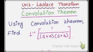
Convolution Theorem
Enroll to start learning
You’ve not yet enrolled in this course. Please enroll for free to listen to audio lessons, classroom podcasts and take practice test.
Interactive Audio Lesson
Listen to a student-teacher conversation explaining the topic in a relatable way.
Introduction to Convolution and its Definition
🔒 Unlock Audio Lesson
Sign up and enroll to listen to this audio lesson

Today, we're going to explore the Convolution Theorem. What do you think convolution means in this context?

Isn’t convolution about combining two functions?
Exactly! Convolution blends two functions through a specified integral. Formally, for two functions f(t) and g(t), it's defined as (f ∗ g)(t).

So, how does this integral look?
Good question! It's given by: \[ (f ∗ g)(t) = \int_0^t f(\tau) g(t - \tau) d\tau \]. This combination represents how one function modifies the other over time.

What does it mean to flip and shift a function?
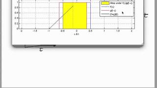
To visualize convolution, think of flipping one function and then shifting it along the other to compute the extent of their overlap. This operation helps in understanding their combined effect.

Got it! It’s like blending sounds in music.
Great analogy! In essence, convolution allows us to see how the inputs affect the outputs — a principle crucial in engineering contexts.
To summarize, convolution is an integral operation that combines functions, and it's denoted as (f ∗ g)(t), represented by the integral of their product over a shifting parameter.
Convolution Theorem for Laplace and Fourier Transforms
🔒 Unlock Audio Lesson
Sign up and enroll to listen to this audio lesson

Next, let's discuss how convolution connects to Laplace and Fourier transforms. Can anyone explain what the Laplace transform does?
It converts a time-domain function into a frequency-domain function!
Exactly! Now, when we apply the Convolution Theorem, if F(s) = L{f(t)} and G(s) = L{g(t)} then what do we get?
Oh, we get L{(f ∗ g)(t)} = F(s)·G(s)! That’s multiplication in the s-domain.
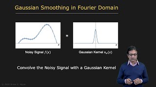
Correct! And similarly, for Fourier Transforms we have: F{f ∗ g}(ω) = F(ω)·G(ω), right?
Right! So convolution in time translates to multiplication in frequency?
Exactly! This theorem is invaluable for simplifying complex analyses in engineering problems.
How does this apply in real-world engineering?
Great question! For example, in structural dynamics, it helps predict how structures respond to various forces over time by simplifying calculations between domains.
To wrap up, we’ve covered how convolution relates to both Laplace and Fourier transforms and significantly simplifies our analyses.
Properties of Convolution
🔒 Unlock Audio Lesson
Sign up and enroll to listen to this audio lesson
Let’s dive into the properties of convolution. Why do you think these properties are important?
They might help us simplify calculations or ensure consistency between functions?
"Absolutely! The properties include:
Applications of Convolution in Civil Engineering
🔒 Unlock Audio Lesson
Sign up and enroll to listen to this audio lesson
Now, let's explore the various applications of convolution in Civil Engineering. Why do you think convolution is essential for structural analysis?
It sounds like it helps in predicting how structures will respond to changing loads!
Correct! Convolution allows us to model the response over time due to dynamic loads, essential for earthquake analysis.
What about heat transfer? How is that connected?
In heat transfer, the temperature distribution can be expressed as a convolution of the heat input function with the system’s impulse response.
This applies to groundwater flow too, right?
Definitely! In hydrology, convolution assists in solving flow problems, particularly in porous media.
What about vibrations in engineering systems?
Vibrations can be analyzed using convolution with Green's functions, helping us understand damped vibrating systems like bridges and buildings.
In summary, convolution is widely applicable in structural analysis, heat transfer, groundwater flow, and vibrations, providing essential insights across Civil Engineering disciplines.
Introduction & Overview
Read summaries of the section's main ideas at different levels of detail.
Quick Overview
Standard
The Convolution Theorem is a foundational concept in Fourier and Laplace Transforms that simplifies the analysis of systems by relating the convolution of two functions in the time domain to their multiplication in the frequency domain. It finds applications in diverse fields, particularly in Civil Engineering, for analyzing structural dynamics, heat transfer, and fluid flow.
Detailed
Detailed Summary of the Convolution Theorem
The Convolution Theorem provides a powerful tool in the fields of Fourier and Laplace transforms, facilitating the evaluation of the transform of the product of two functions. This theorem is critical in various engineering applications, particularly in Civil Engineering, where it aids in solving linear systems, integral equations, and differential equations essential for structural analysis, heat transfer, and dynamic loading conditions.
- Definition of Convolution: The convolution of two piecewise continuous functions, denoted as
(f ∗ g)(t), is defined by the integral:
\[ (f ∗ g)(t) = \int_0^t f(\tau)g(t - \tau) d\tau \]
- Key Theorems: For Laplace Transforms, the theorem states that if F(s) = L{f(t)} and G(s) = L{g(t)}, then:
\[ L\{(f ∗ g)(t)\} = F(s) \, G(s) \]
In the context of Fourier Transforms, it implies:
\[ F\{f ∗ g\}(\omega) = F(\omega) \, G(\omega) \]
- Properties of Convolution: Important properties include commutativity, associativity, distributive over addition, and the existence of an identity element (the Dirac delta function).
- Applications: Convolution has significant applications in Civil Engineering including structural analysis, heat transfer in materials, groundwater flow, and vibrations in beams and plates.
- Solving Differential Equations: The convolution is instrumental in solving linear differential equations, particularly through using laplace transforms to yield solutions in time domain.
In conclusion, understanding the Convolution Theorem enhances engineers' ability to model and analyze systems effectively, establishing a crucial link between time and frequency domains.
Youtube Videos

Audio Book
Dive deep into the subject with an immersive audiobook experience.
Introduction to the Convolution Theorem
Chapter 1 of 6
🔒 Unlock Audio Chapter
Sign up and enroll to access the full audio experience
Chapter Content
The Convolution Theorem is a powerful result in the theory of Fourier Transforms and Laplace Transforms. It simplifies the process of evaluating the transform of a product of two functions. In the context of engineering, especially Civil Engineering, it is particularly useful for solving linear systems, integral equations, and differential equations encountered in structural analysis, fluid flow, heat transfer, and vibration problems.
Detailed Explanation
The Convolution Theorem provides a simplified way to handle the Fourier and Laplace Transforms of products of functions. It is especially important in engineering disciplines where systems can often be described mathematically through linear functions. The theorem helps in transforming complex products into simpler multiplicative forms, enabling engineers to effectively analyze and solve equations related to systems dynamics.
Examples & Analogies
Imagine you're mixing two colors of paint to create a new shade. Each color has its own properties (like brightness and saturation), and when you mix them, the result has its unique characteristics, just like how convolution blends two functions to understand the effect of one on the other.
Definition of Convolution
Chapter 2 of 6
🔒 Unlock Audio Chapter
Sign up and enroll to access the full audio experience
Chapter Content
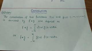
Let f(t) and g(t) be two piecewise continuous functions defined for t≥0. The convolution of f and g, denoted by (f ∗g)(t), is defined as:
Z t
(f ∗g)(t)= f(τ)g(t−τ)dτ
0
This definition is symmetric in f and g, meaning:
(f ∗g)(t)=(g∗f)(t).
Detailed Explanation
Convolution involves integrating the product of two functions where one function is reversed and shifted. The notation (f ∗g)(t) represents this operation, and the equation shows how to compute it using integration from 0 to t. The symmetry indicates that the order in which you convolve the functions does not matter—(f ∗g) is the same as (g ∗f).
Examples & Analogies
Consider two waves in water intersecting: one wave might represent the wind's influence (f) while the other represents a boat's movement (g). When they combine (convolve), the resulting wave pattern shows how the boat is affected by the wind over time.
Convolution Theorem for Laplace Transforms
Chapter 3 of 6
🔒 Unlock Audio Chapter
Sign up and enroll to access the full audio experience
Chapter Content
If F(s) = L{f(t)} and G(s) = L{g(t)}, then the Laplace transform of their convolution is:
L{(f ∗g)(t)}=F(s)·G(s).
This relationship shows that performing convolution in the time domain translates into multiplication in the Laplace domain.
Detailed Explanation
The theorem states that the Laplace transform of the convolution of two functions equals the product of their individual Laplace transforms. This property is significant because it allows engineers and mathematicians to work in the simpler multiplicative realm of transforms rather than directly dealing with convolutions in the time domain, which can be complicated and cumbersome.
Examples & Analogies
Think of it like cooking: if you know two separate recipes (like F(s) and G(s)), but instead of making each dish separately (the convolution), you realize that by combining the ingredients (multiplying), you can save time and effort.
Convolution Theorem for Fourier Transforms
Chapter 4 of 6
🔒 Unlock Audio Chapter
Sign up and enroll to access the full audio experience
Chapter Content
Let f(t), g(t) ∈ L1(R), and let their Fourier transforms be F(ω) and G(ω). Then:
F{f ∗g}(ω)=F(ω)·G(ω).
And conversely:
F^{-1}{F(ω)·G(ω)}(t)=(f ∗g)(t).
Detailed Explanation
This part of the theorem establishes a relationship between convolution in the time domain and multiplication in the frequency domain. It illustrates the dual nature of convolution and multiplication across the transforms, showing how they interrelate in analysis, allowing for easier interpretations of systems' frequency behavior.
Examples & Analogies
Imagine you're tuning a radio to catch a specific station. The signals you pick up from the antenna can be thought of as convolutions of many different frequencies. By filtering out certain frequencies (multiplying), you isolate the music you want to hear, just like how the theorem helps to isolate and analyze components of signals.
Properties of Convolution
Chapter 5 of 6
🔒 Unlock Audio Chapter
Sign up and enroll to access the full audio experience
Chapter Content
- Commutative Property: f∗g=g∗f
- Associative Property: (f∗g)∗h=f∗(g∗h)
- Distributive over Addition: f∗(g+h)=f∗g+f∗h
- Identity Element: The Dirac delta function δ(t) acts as the identity: f∗δ=f.
Detailed Explanation
These properties confirm that convolution operations maintain certain predictable characteristics that are useful in mathematical manipulations. For example, the commutative property tells us that the order in which we convolve two functions doesn’t change the result, similar to addition.
Examples & Analogies
Think of mixing ingredients: It doesn’t matter if you add flour to sugar or sugar to flour, the final mix will have the same taste and texture (commutative). If you think of a recipe that combines multiple ingredients, the order of mixing doesn’t change the final cake either (associative).
Applications in Civil Engineering
Chapter 6 of 6
🔒 Unlock Audio Chapter
Sign up and enroll to access the full audio experience
Chapter Content
- Structural Analysis: Convolution can model how structures respond over time to varying loads — crucial in earthquake analysis and dynamic loading conditions.
- Heat Transfer: Temperature distribution in slabs or columns subject to variable heat sources can be expressed as a convolution of the input (heat function) with the system's impulse response.
- Groundwater Flow: In hydrology, convolution helps solve flow problems in porous media, especially in estimating response functions to precipitation input.
- Vibrations of Beams and Plates: The response of damped vibrating systems (common in bridges and buildings) to external forces is found using convolution with Green’s function or impulse responses.
Detailed Explanation
These applications highlight the versatility of convolution in solving real-world engineering challenges. By applying convolution, engineers can predict how systems respond over time to various stimuli—loads, temperature changes, and even environmental conditions. This is particularly vital in maintaining safety and efficiency in designs.
Examples & Analogies
Consider the way your house reacts to rain. When heavy rain falls, it’s not just the immediate weight of water but how that load changes over time that affects structural integrity. Engineers use convolution to predict those changes and ensure safety, much like preparing for potential flooding by improving drainage systems.
Key Concepts
-
Convolution: A way of blending two functions, represented by an integral.
-
Transformations: The relationship between time-domain convolution and frequency-domain multiplication.
-
Commutative Property: Order of functions does not affect convolution.
-
Impulse Response: The system's response when it encounters a brief input signal.
Examples & Applications
Evaluating the convolution of f(t) = t and g(t) = e^(-t).
Solving a second-order linear ordinary differential equation using convolution involving the impulse response.
Memory Aids
Interactive tools to help you remember key concepts
Rhymes
Convolution's a blend, try to comprehend, one flips and shifts, as the functions mix.
Stories
Imagine two rivers, f(t) and g(t), flowing together in a way that the height of one modifies the other, creating a new river called (f ∗ g)(t).
Memory Tools
Remember the acronym 'CAMP': C for Commutative, A for Associative, M for Multiplication (in the transformed domain), and P for Properties.
Acronyms
The acronym 'LFT' can help you remember
'L' for Laplace
'F' for Fourier
'T' for Theorem.
Flash Cards
Glossary
- Convolution
An operation that combines two functions to produce a third function, representing how one function modifies another.
- Laplace Transform
An integral transform that converts a time-domain function into a complex frequency domain representation.
- Fourier Transform
A mathematical transform that decomposes a function into its constituent frequencies.
- Piecewise Continuous Functions
Functions that are continuous over intervals but may be defined in pieces.
- Impulse Response
The response of a system to a brief input signal, forming the basis for the convolution in system analysis.
- Dirac Delta Function
A mathematical construct that represents an idealized point mass or point charge; it acts as the identity element in convolution.
Reference links
Supplementary resources to enhance your learning experience.