
Solving Differential Equations Using Convolution
Enroll to start learning
You’ve not yet enrolled in this course. Please enroll for free to listen to audio lessons, classroom podcasts and take practice test.
Interactive Audio Lesson
Listen to a student-teacher conversation explaining the topic in a relatable way.
Introduction to Differential Equations and Convolution
🔒 Unlock Audio Lesson
Sign up and enroll to listen to this audio lesson

Today, we're going to cover how we can use convolution to solve differential equations. Can anyone tell me what a differential equation is?

Isn't it an equation that relates a function with its derivatives?
Exactly right! Now, who can give an example of a second-order differential equation?

Like \( y'' + ay' + by = f(t) \)?
Nice job! Now, we'll see how convolution simplifies solving such equations. Shall we then move on to the next step?
Laplace Transform Basics
🔒 Unlock Audio Lesson
Sign up and enroll to listen to this audio lesson

When we take the Laplace Transform of our differential equation, it turns into an algebraic equation. Does anyone know what \( Y(s) \) represents?

It's the Laplace Transform of \( y(t) \)!
Correct! And we also have \( F(s) \) for the Laplace Transform of our function \( f(t) \). Now, let’s see how we manipulate the equation from there.
So we solve for \( Y(s) \) to get our solution in the Laplace domain?
Exactly! Remember, once we find \( Y(s) \), we must convert it back to the time domain using the inverse Laplace Transform. Let's proceed with the next part.
Using Convolution to Solve Differential Equations
🔒 Unlock Audio Lesson
Sign up and enroll to listen to this audio lesson
Here's where convolution comes into play! We express our solution as \( y(t) = (f * h)(t) \). What does \( h(t) \) represent?
It's the impulse response of the system!
Correct! It tells us how the system responds to an impulse over time. Can someone summarize how we use this in practice?

We find the inverse Laplace Transform of \( \frac{1}{s^2 + as + b} \) to get \( h(t) \), then we convolve it with \( f(t) \)!
Well done! This method greatly simplifies our calculations in engineering contexts. Let's move to a real-world example.
Example of Solving a Differential Equation
🔒 Unlock Audio Lesson
Sign up and enroll to listen to this audio lesson
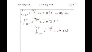
Let’s apply what we learned. Consider the equation \( y'' + y = ext{sine}(t) \) with initial conditions. How would we start solving this?
First, we would take the Laplace Transform!
Correct! After the transform, what does our equation look like?
It's \( Y(s)(s^2 + 1) = \frac{1}{s} \), right?
Exactly! So how do we find \( y(t) \) from here?
We solve for \( Y(s) \) and find its inverse Laplace Transform?
That's it! Following that, we can apply the convolution method to find the complete solution. Great work today, everyone!
Introduction & Overview
Read summaries of the section's main ideas at different levels of detail.
Quick Overview
Standard
Convolution provides an efficient method for solving differential equations by transforming them into algebraic equations using Laplace Transforms, and utilizing the impulse response to find solutions. This section illustrates the process with equations and an example.
Detailed
Detailed Summary
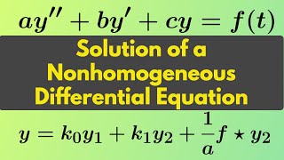
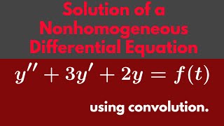
In this section, we explore the application of convolution in solving second-order linear ordinary differential equations of the form:
\[ y'' + ay' + by = f(t) \]
We begin by taking the Laplace Transform of both sides, using initial conditions to simplify our equation. The transformed equation looks like:
\[ s^2Y(s) + asY(s) + bY(s) = F(s) + \text{initial terms} \]
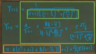
This allows us to solve for \( Y(s) \):
\[ Y(s) = \frac{F(s) + \text{terms from initial conditions}}{s^2 + as + b} \]
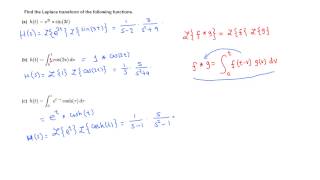
Next, we use convolution to express the solution in the time domain:
\[ y(t) = (f * h)(t) \]
where \( h(t) \) is the inverse Laplace Transform of \( \frac{1}{s^2 + as + b} \), representing the system's impulse response. This technique ties together the concept of convolution with practical applications in engineering, making it a vital tool in analyzing and solving differential equations.
Youtube Videos
Audio Book
Dive deep into the subject with an immersive audiobook experience.
The Differential Equation Setup
Chapter 1 of 4
🔒 Unlock Audio Chapter
Sign up and enroll to access the full audio experience
Chapter Content
Consider a second-order linear ordinary differential equation with initial conditions:
y′′+ay′+by =f(t)
Detailed Explanation
This initial setup presents a second-order linear ordinary differential equation (ODE) where 'y' is the unknown function, 'a' and 'b' are constants, and 'f(t)' is a function representing external inputs (a forcing function). The prime notation indicates derivatives of 'y' with respect to time. This equation models many physical systems and phenomena, including mechanical vibrations and electrical circuit responses.
Examples & Analogies
Think of a swing in a playground. The forces acting on it (like someone pushing the swing) can be modeled as 'f(t)', the initial position and speed of the swing represent the initial conditions, and the formulas help predict how high and how far the swing will go over time.
Applying the Laplace Transform
Chapter 2 of 4
🔒 Unlock Audio Chapter
Sign up and enroll to access the full audio experience
Chapter Content
Taking Laplace Transform and applying initial conditions:
s²Y(s)+asY(s)+bY(s)=F(s)+initial terms
Detailed Explanation
The Laplace Transform converts the differential equation into an algebraic equation in the 's' domain, which is often easier to work with. Here, 'Y(s)' is the Laplace Transform of 'y(t)', and 'F(s)' represents the Laplace Transform of the forcing function 'f(t)'. The initial conditions provide the necessary values to solve for 'Y(s)' completely.
Examples & Analogies
Imagine translating a recipe (the differential equation) into a simpler form to understand the steps (algebraic equation) without having to worry about timing and cooking methods. The Laplace Transform simplifies the process, making it easier to arrive at a solution.
Solving for Y(s)
Chapter 3 of 4
🔒 Unlock Audio Chapter
Sign up and enroll to access the full audio experience
Chapter Content
Solving for Y(s):
Y(s)=F(s)+terms from initial conditions
(s²+as+b)
Detailed Explanation
In rearranging the transformed equation, Y(s) is isolated on one side. This equation expresses Y(s) as a combination of the transformed input function F(s) and terms derived from initial conditions, divided by a polynomial related to the system characteristics (represented as (s² + as + b)). This step is crucial for finding the solution in the time domain later.
Examples & Analogies
Consider a problem where you need to calculate the final height of a structure but first need to consider its foundation and materials. Here, the denominator (s² + as + b) represents the foundation, while F(s) includes the external forces acting upon it, showing how all factors influence the final outcome.
Using Convolution for the Solution
Chapter 4 of 4
🔒 Unlock Audio Chapter
Sign up and enroll to access the full audio experience
Chapter Content
Now, using convolution:
y(t)=(f ∗h)(t)
Where h(t) is the inverse Laplace Transform of 1/(s²+as+b) which acts as the impulse response.
Detailed Explanation
The solution y(t) is expressed as the convolution of the input function f(t) and the impulse response h(t). The impulse response is derived from the inverse Laplace Transform of the polynomial in the denominator, allowing for the effect of the initial conditions and the external forcing function to be combined to provide the overall response of the system over time. This convolution encapsulates how the system reacts to the inputs throughout its time evolution.
Examples & Analogies
Imagine playing with a trampoline. When you jump (f(t)), the trampoline's response (h(t)) depends on how springy and bouncy it is. The overall bounce you feel as you jump at different times is like the convolution, combining your action and the trampoline's reaction to give a complete view of your bouncing experience.
Key Concepts
-
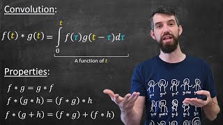
Convolution: A powerful technique for combining functions that helps solve differential equations.
-
Laplace Transform: A method for transforming differential equations into algebraic form.
-
Impulse Response: Represents the effect of an impulse on the system over time.
Examples & Applications
Example of solving a differential equation, demonstrating the use of Laplace Transforms and convolution.
Convolution applied to find the output of linear systems given an input function.
Memory Aids
Interactive tools to help you remember key concepts
Rhymes
When a force takes a sudden bend, convolution helps us comprehend!
Stories
Imagine a calm lake—throw a stone (impulse). Watch the ripples (response) travel and spread, that's how convolution shapes the impact of an input on a system over time.
Memory Tools
Remember 'C-LIP': Convolution-Laplace Impulse Response for solving equations.
Acronyms
Use 'CIR' to recall
Convolution Is Response when dealing with systems.
Flash Cards
Glossary
- Convolution
A mathematical operation that combines two functions to produce a third function, representing how the shape of one function is modified by another.
- Laplace Transform
A technique used to transform a function of time into a function of a complex variable, simplifying the process of solving differential equations.
- Impulse Response
The output response of a system when an impulse is applied at time zero.
- SecondOrder Differential Equation
An equation that involves the second derivative of a function and may include the first derivative of the same function.
Reference links
Supplementary resources to enhance your learning experience.