
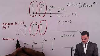
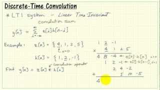
Example 4: Discrete-Time Convolution
Enroll to start learning
You’ve not yet enrolled in this course. Please enroll for free to listen to audio lessons, classroom podcasts and take practice test.
Interactive Audio Lesson
Listen to a student-teacher conversation explaining the topic in a relatable way.
Introduction to Discrete-Time Convolution
🔒 Unlock Audio Lesson
Sign up and enroll to listen to this audio lesson

Today, we will discuss discrete-time convolution, a crucial concept in digital signal processing. Can anyone tell me why we use convolution in discrete systems?

Isn't it used to analyze signals and filter responses?
Exactly! We convolve signals to see how one influences the other over time. The key idea is to combine two sequences to produce a new one that reflects their interaction.

How do we actually perform the convolution?
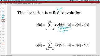
Great question! We use the formula (f ∗ g)[n] = Σ f[k] * g[n - k]. This means we'll calculate the sum of products for all overlapping indices.
Calculating Discrete-Time Convolution
🔒 Unlock Audio Lesson
Sign up and enroll to listen to this audio lesson

Let’s look at our example: f[n] = {1, 2, 1} and g[n] = {1, 1}. For n=0, can anyone compute (f ∗ g)[0]?

For n=0, I think it would be f[0]*g[0] = 1*1 = 1.
Correct! Now for n=1, we need to consider where both sequences overlap. What do you calculate for n=1?

(f ∗ g)[1] = f[0]*g[1] + f[1]*g[0] = 1*1 + 2*1, which is 1 + 2 = 3.
Well done! Now, let's keep this momentum going. What about n=2?
Continuing the Convolution Calculation
🔒 Unlock Audio Lesson
Sign up and enroll to listen to this audio lesson
So far, we have (f ∗ g)[0] = 1 and (f ∗ g)[1] = 3. Next, let’s calculate (f ∗ g)[2]. Who wants to give it a try?
For n=2, I think we add f[0]*g[2], f[1]*g[1], and f[2]*g[0]. It looks like we treat g[2] as 0 since it’s outside the range of g.
Then we have 0 + 2*1 + 1*1, which equals 3.
Great! Moving on, what happens for n=3?
(f ∗ g)[3] = f[1]*g[2] + f[2]*g[1]. But again, g[2] is 0, so we have 0 + 1*1 = 1.
Perfect! So we conclude that (f ∗ g)[n] = {1, 3, 3, 1}. Can anyone summarize why convolution is useful?
Significance and Applications of Discrete-Time Convolution
🔒 Unlock Audio Lesson
Sign up and enroll to listen to this audio lesson
Now that we've computed the result of the convolution, let's talk about its significance. Why is understanding convolution in a digital context important?
Because it helps in signal processing applications like filtering and system behavior analysis.
Exactly! It's essential for understanding how various inputs affect a system's output over time.
How can we further apply this knowledge in civil engineering?
Well, convolution can be used in analyzing vibrations in structures. By convolving a force input with a system's impulse response, we can understand how that force influences the structure through time.
Introduction & Overview
Read summaries of the section's main ideas at different levels of detail.
Quick Overview
Standard
Discrete-time convolution is a vital operation in digital signal processing, allowing the analysis of signals. This section includes a detailed example illustrating the steps for calculating the convolution of two discrete sequences.
Detailed
In this section on discrete-time convolution, we focus on the convolution of two sequences, f[n] = {1, 2, 1} and g[n] = {1, 1}. The convolution is computed through a systematic summation process, evaluating the contribution at each index. The methodology relies on the definition of convolution for discrete signals, where the result at index n is derived from the sum of products of the functions over a range of indices. The final result of the convolution, (f ∗ g)[n], is {1, 3, 3, 1}, demonstrating how the convolution operation combines the characteristics of both sequences across their lengths.
Youtube Videos

Audio Book
Dive deep into the subject with an immersive audiobook experience.
Introduction to Discrete-Time Convolution
Chapter 1 of 6
🔒 Unlock Audio Chapter
Sign up and enroll to access the full audio experience
Chapter Content
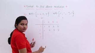
Given:
f[n]={1,2,1}, g[n]={1,1}
Find (f ∗g)[n].
Detailed Explanation
In this example, we are given two discrete functions: f[n] = {1, 2, 1} and g[n] = {1, 1}. The goal is to find the convolution of these two functions, denoted as (f ∗ g)[n]. This involves calculating the values of (f ∗ g)[n] for different values of n, which represents the time index in discrete-time systems. The convolution operation combines these two sequences into a new sequence that describes how the input signal f interacts with the filter g over time.
Examples & Analogies
Think of f[n] and g[n] as two different sequences of events, like two different musical melodies played over a set amount of time. The convolution would represent how these two melodies blend together to create a new sound, with notes overlapping according to the timing and strength of each note in the original melodies.
Calculating Convolution for n=0
Chapter 2 of 6
🔒 Unlock Audio Chapter
Sign up and enroll to access the full audio experience
Chapter Content
• n=0: f[0]g[0]=1·1=1
Detailed Explanation
For n = 0, we are looking at the first index of the sequences. We compute the convolution by multiplying f[0] with g[0]. Here, f[0] = 1 and g[0] = 1, thus (f ∗ g)[0] equals 1. This is a straightforward case where both sequences have non-zero values at their starting positions.
Examples & Analogies
Imagine you are mixing two paints starting with their first drops. If the first drop of paint from f is red (1) and the first drop of paint from g is blue (1), when you mix them together you simply get a small amount of the mixed color (1) right at the beginning.
Calculating Convolution for n=1
Chapter 3 of 6
🔒 Unlock Audio Chapter
Sign up and enroll to access the full audio experience
Chapter Content
• n=1: f[0]g[1]+f[1]g[0]=1·1+2·1=3
Detailed Explanation
For n = 1, we compute the convolution by taking contributions from f[0] with g[1] and f[1] with g[0]. Here, f[0] = 1, g[1] = 1, f[1] = 2, and g[0] = 1. Therefore, we find (f ∗ g)[1] = (1 * 1) + (2 * 1) = 3. This shows how elements at different time indices combine during convolution.
Examples & Analogies
Imagine you're adding ingredients to a recipe. For n=1, you're combining the first ingredient and the second ingredient of two different recipes: one recipe calls for 1 cup of flour (f[0]) and the other for 2 cups of sugar (f[1]). When each aspect from one recipe is combined with another (1 cup of flour with 1 cup of sugar), you end up with a total of 3 units of mixed ingredients (3).
Calculating Convolution for n=2
Chapter 4 of 6
🔒 Unlock Audio Chapter
Sign up and enroll to access the full audio experience
Chapter Content
• n=2: f[0]g[2]+f[1]g[1]+f[2]g[0]=0+2·1+1·1=3
Detailed Explanation
For n = 2, the convolution is calculated by considering contributions from multiple indices. Here, g[2] is 0 (as g[n] only has values for n=0 and n=1), so its contribution is zero. Thus, we focus on the non-zero contributions from f[1] and f[2]: (f ∗ g)[2] = (0 * 1) + (2 * 1) + (1 * 1) = 3. This reflects how the convolution integrates overlapping values to create the new output.
Examples & Analogies
Imagine four friends at a gathering, where you’re counting interactions based on an event timeline. For n=2, the interaction between a few friends from two different circles creates a combined score of 3 because not all groups are present at the same time (one group is missing), but those who are present can still connect and result in meaningful interactions, like friendships.
Calculating Convolution for n=3
Chapter 5 of 6
🔒 Unlock Audio Chapter
Sign up and enroll to access the full audio experience
Chapter Content
• n=3: f[1]g[2]+f[2]g[1]=0+1·1=1
Detailed Explanation
For n = 3, we compute the values using f[1] and g[2], and f[2] and g[1]. Since g[2] is outside the bounds of g[n], its value is 0, so we have (f ∗ g)[3] = (0 * 1) + (1 * 1) = 1. This final calculation shows how only one term contributes to the output, illustrating how convolution captures the essence of overlapping signals even in sparse cases.
Examples & Analogies
Think about a performance with last-minute guests arriving. For n=3, the combination of someone arriving at just the right time with one solo performer results only in a single collaboration (1) because only they interacted directly, and everyone else was either busy or away!
Final Output of Discrete-Time Convolution
Chapter 6 of 6
🔒 Unlock Audio Chapter
Sign up and enroll to access the full audio experience
Chapter Content
Hence, (f ∗g)[n]={1,3,3,1}
Detailed Explanation
The final result of our convolution operation, (f ∗ g)[n] = {1, 3, 3, 1}, summarizes how f and g interacted across all time indices. Each number represents the strength or magnitude of the output signal at that specific time based on the blending of the two original signals. It shows how signals contribute over time, providing an important outcome in the context of signal processing.
Examples & Analogies
Visualize a coaching session in sports where each player's performance (made of sequences of points scored over different time intervals) blends into the team's total score. The final score reflects contributions from all players, cumulatively layered together into a remarkable performance score (1, 3, 3, 1), demonstrating not just individual values but the strength of collaborative effort over time.
Key Concepts
-
Sum of Products: The core of discrete convolution is the sum of products of overlapping values of two signals.
-
Index Shift: Each discrete convolution output corresponds to an index shift in one of the input sequences.
Examples & Applications
Calculating (f∗g)[0]: For n=0, it's f[0]*g[0] = 1.
Conclusion of convolution result: (f∗g)[n] = {1, 3, 3, 1}.
Memory Aids
Interactive tools to help you remember key concepts
Rhymes
Convolve the functions near, sum them up without fear!
Stories
Imagine f is a person throwing a ball, while g is a wall. The path of the ball changes with each bounce off the wall, just like how signals influence each other in convolution.
Memory Tools
FUSE: For Understanding Signals Everywhere - remember to fuse signals through convolution!
Acronyms
C.O.N.V.O.L.V.E - Calculate Overlapping Numbers Via Online Logic in Variables Everywhere.
Flash Cards
Glossary
- DiscreteTime Convolution
An operation that combines two discrete signals to form a third signal, representing how one signal influences the other.
- Impulse Response
The output of a system when presented with a brief input or impulse signal; it characterizes the response of a system.
Reference links
Supplementary resources to enhance your learning experience.