
Example 3: Piecewise Convolution
Enroll to start learning
You’ve not yet enrolled in this course. Please enroll for free to listen to audio lessons, classroom podcasts and take practice test.
Interactive Audio Lesson
Listen to a student-teacher conversation explaining the topic in a relatable way.
Understanding the Functions
🔒 Unlock Audio Lesson
Sign up and enroll to listen to this audio lesson

Today, we will begin by analyzing two functions: f(t) and g(t). Can anyone explain what a piecewise function is?

A piecewise function is defined by different expressions based on the input value, right?
Exactly! So, for our piecewise functions, f(t) is defined as 1 for t between 0 and 1. What about g(t)?

g(t) is just t, but that means it increases linearly across its range.
Right! Understanding the definitions is crucial since they'll guide us in computing the convolution.
Calculating the Convolution
🔒 Unlock Audio Lesson
Sign up and enroll to listen to this audio lesson

Let's write down the convolution integral. Who remembers the formula?

It's the integral of f(τ)g(t-τ) dτ from 0 to t, right?
Correct! Now, how do we set this up for our specific functions regarding their ranges?

We consider t values separately! For 0 ≤ t ≤ 1, both functions behave differently compared to when t > 1.
Exactly! Let's work through Case 1 and establish what (f ∗ g)(t) is for that range.
Case Analysis
🔒 Unlock Audio Lesson
Sign up and enroll to listen to this audio lesson
Now, we've calculated the convolution for t in the first case. What do we get?
We find (f ∗ g)(t) = t²/2 for 0 ≤ t ≤ 1!
Perfect! But now, what changes for t > 1?
Then we only consider f(τ) from 0 to 1 due to its piecewise definition.
Exactly! Now verifying this integration, we can derive the second part: t - 1/2. What does that lead us to?
We can compile both results into a piecewise function!
Final Conclusion
🔒 Unlock Audio Lesson
Sign up and enroll to listen to this audio lesson
Alright, can we summarize the final piecewise result that we obtained?
Sure! (f ∗ g)(t) = t²/2 for 0 ≤ t ≤ 1 and t - 1/2 for t > 1!
Well articulated! This clearly demonstrates how function behavior affects convolution. Well done!
Introduction & Overview
Read summaries of the section's main ideas at different levels of detail.
Quick Overview
Standard
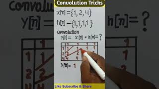
In this section, we explore the example of piecewise convolution between two functions: f(t), defined as 1 for 0≤t≤1, and g(t), defined as t for the same interval. The convolution is computed for two cases, where the ranges of t differ, illustrating the integral calculations distinctly for the two scenarios.
Detailed
Example 3: Piecewise Convolution
In this section, we analyze the convolution of two piecewise functions, f(t) and g(t), specifically designed to demonstrate how piecewise definitions impact the convolution process:
- f(t) is defined as:
$$
f(t) = \begin{cases}
1, & 0 \leq t \leq 1 \
0, & t > 1
\end{cases}
$$
- g(t) is defined as:
$$
g(t) = t
$$
The goal is to compute the convolution of f and g, symbolized as (f ∗ g)(t).
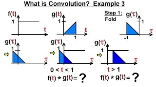
Finding (f ∗ g)(t)
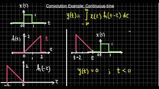
The formula for convolution is given by:
$$
(f ∗ g)(t) = \int_{0}^{t} f(\tau)g(t - \tau)d\tau
$$
In solving this, we need to consider two scenarios based on the piecewise nature of f(t):
- Case 1: 0 ≤ t ≤ 1
- For this scenario, f(\tau) equals 1 for all \tau within the limits of integration:
$$
(f ∗ g)(t) = \int_{0}^{t} (1)(t - \tau) d\tau = \int_{0}^{t} (t - \tau) d\tau
$$
- Evaluating this integral yields:
$$
(f ∗ g)(t) = \left[ t\tau - \frac{\tau^2}{2} \right]_{0}^{t} = tt - \frac{t^2}{2} = \frac{t^2}{2}
$$
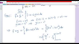
- Case 2: t > 1
- In this case, f(\tau) remains equal to 1 only from τ=0 to τ=1. Therefore, the limits of the integral adjust accordingly:
$$
(f ∗ g)(t) = \int_{0}^{1}(1)(t - \tau) d\tau = \left[ t\tau - \frac{\tau^2}{2} \right]_{0}^{1}
$$
- This results in:
$$
(f ∗ g)(t) = (t)(1) - \frac{(1)^2}{2} = t - \frac{1}{2}
$$
Piecewise Result
Combining both cases, we can express the final result of the convolution as a piecewise function:
$$
(f ∗ g)(t) = \begin{cases}
\frac{t^2}{2}, & 0 \leq t \leq 1 \
t - \frac{1}{2}, & t > 1
\end{cases}
$$
This example illustrates the importance of considering the nature of the functions when performing convolution, particularly when applying it to real-world engineering scenarios.
Youtube Videos

Audio Book
Dive deep into the subject with an immersive audiobook experience.
Defining Functions f(t) and g(t)
Chapter 1 of 4
🔒 Unlock Audio Chapter
Sign up and enroll to access the full audio experience
Chapter Content
Let:
$$
f(t)=\begin{cases}
1, & 0 \leq t \leq 1 \
0, & t > 1
\end{cases}$$
$$
g(t)=t$$
Detailed Explanation
In this example, we have two functions. The function f(t) is defined as 1 between time 0 and 1, and 0 afterwards, which means it only has a significance in that small time window. On the other hand, g(t) is simply the function that equals t, meaning its value increases constantly as time progresses. These functions will be used to calculate their convolution over different time intervals.
Examples & Analogies
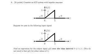
Imagine f(t) as a light switch that is turned on (value 1) only for the first second of a process, representing a brief burst of energy, while g(t) represents a continuously increasing temperature gauge. During the brief moment when the switch is on, we will analyze how that quick burst affects the temperature gauge over time.
Calculating the Convolution for Case 1 (0 ≤ t ≤ 1)
Chapter 2 of 4
🔒 Unlock Audio Chapter
Sign up and enroll to access the full audio experience
Chapter Content
We compute:
$$
\int_0^t (f \ast g)(t)= \int_0^t f(\tau) g(t-\tau) d\tau
$$
Since f(\tau)=1 for \tau \in[0,t]:
$$
\int_0^t (t-\tau) d\tau = \frac{t^2}{2}$$
Detailed Explanation
In this case (when t is between 0 and 1), we substitute f(τ) = 1, simplifying our integral to just g(t - τ) over the range from 0 to t. This results in the integral that computes the area under the graph of g(t) from 0 to t, giving us \( \frac{t^2}{2} \), which captures the cumulative effect of g(t) during this time period.
Examples & Analogies
Think of this as pouring a little bit of syrup (g(t)) into a container (the integral) every second for the first one second. The total volume of syrup collected in that second is represented by \( \frac{t^2}{2} \) - showing how much can accumulate even in that short burst.
Calculating the Convolution for Case 2 (t > 1)
Chapter 3 of 4
🔒 Unlock Audio Chapter
Sign up and enroll to access the full audio experience
Chapter Content
Now f(\tau)=1 only from \tau =0 to 1:
$$
\int_0^1 (t-\tau) d\tau = t\tau - \frac{\tau^2}{2} \Big|_0^1 = t - \frac{1}{2}$$
Detailed Explanation
In this case (when t is greater than 1), f(τ) remains 1 only from 0 to 1, while g(t - τ) adjusts accordingly. The integral thus computes the area under g(t) again, but this time the upper limit of the integral is capped at 1, reflecting that f(τ) is not active beyond that point. The result is \( t - \frac{1}{2} \), indicating how the initial burst (from f(t)) has an effect even after it has turned off.
Examples & Analogies
Imagine a hose (g(t)) which starts spraying water continuously after the switch is pushed. Even after the brief activation of the switch, the water sprays for a while, but it is limited by the initial pressure (1 unit of f(τ)) established only for a short moment. As time passes beyond that initial burst, the total effect on the system can be computed until the constraints of the burst influence the overall outcome.
Final Results of the Convolution
Chapter 4 of 4
🔒 Unlock Audio Chapter
Sign up and enroll to access the full audio experience
Chapter Content
Thus:
$$
(f \ast g)(t)=\begin{cases}
t^2, & 0 \leq t \leq 1 \
t - \frac{1}{2}, & t > 1\end{cases}$$
Detailed Explanation
The final result encapsulates everything we've discussed in the previous chunks. It summarizes the impact of both functions through time, reflecting how their interactions yield different results depending on the interval being analyzed. During the onset (0 ≤ t ≤ 1), the effect is quadratic due to the consistent influence of f(t). Beyond that, the growth pattern changes due to the diminishing influence of f(t), giving us a linear effect based on the performance of g(t).
Examples & Analogies
This final expression can be seen as the overall temperature perceived in a room where warm energy was rapidly introduced for just a moment. Initially, during the effective input time, the temperature rises quite dramatically, followed by a gradual increase as the room continues to heat with time. By summarizing the impact mathematically, we can better predict and analyze behaviors in a variety of systems.
Key Concepts
-
Piecewise Convolution: The operation defining the output as a combination of integrals based on the definitions of each segment of the functions.
-
Integral Limits: Distinct intervals must be considered based on the piecewise nature of the functions.
Examples & Applications
Example of the convolution of f(t)=1 (0≤t≤1) and g(t)=t, yielding different results based on the value of t.
Memory Aids
Interactive tools to help you remember key concepts
Rhymes
For f(t) that's one in a span, Convolution helps us understand!
Stories
Once, there were functions f and g that only worked together in their defined ranges. They combined through a magical integral to form a new existence.
Memory Tools
Fabulous Integrals Produce Results - Remember that convolution requires integrating each piece appropriately.
Acronyms
CPR (Convolution, Piecewise, Result) - Remember the process of convolution in piecewise functions.
Flash Cards
Glossary
- Convolution
A mathematical operation that blends two functions, such as f(t) and g(t), to produce a new function representing their overlap.
- Piecewise function
A function defined by multiple segments, each applicable to a specific interval of the input variable, often denoted as f(t).
Reference links
Supplementary resources to enhance your learning experience.