
Convolution Theorem for Laplace Transforms
Enroll to start learning
You’ve not yet enrolled in this course. Please enroll for free to listen to audio lessons, classroom podcasts and take practice test.
Interactive Audio Lesson
Listen to a student-teacher conversation explaining the topic in a relatable way.
Introduction to Laplace Transforms
🔒 Unlock Audio Lesson
Sign up and enroll to listen to this audio lesson

Today, we are going to discuss how Laplace transforms operate, particularly focusing on the Convolution Theorem. Does anyone know what a Laplace transform does?

Isn't it a method to convert a function from time domain to frequency domain?
Exactly! It helps us to simplify differential equations by transforming them into algebraic equations. It’s essential in engineering fields like fluid mechanics and structural analysis.

So, what’s the core idea behind the convolution in this context?
Great question! Convolution basically combines two functions in a certain way—imagine manipulating one function with another. Now when we apply the Laplace transform to a convolution, we can relate it to their individual transforms. By the end of this session, you will understand how convolution in the time domain corresponds to multiplication in the Laplace domain.
The Convolution Theorem Explained
🔒 Unlock Audio Lesson
Sign up and enroll to listen to this audio lesson

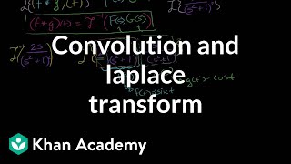
Now let's look at the Convolution Theorem. So, if we have F(s) = L{f(t)} and G(s) = L{g(t)}, the theorem states that the Laplace transform of (f ∗ g)(t) equals F(s) multiplied by G(s). Does anyone want to express this in mathematical notation?

It’s L{(f ∗ g)(t)} = F(s) · G(s).
Exactly! This is a powerful relationship. It implies that’s you don’t have to compute the Laplace transform of a convolution directly—instead, you can transform each function separately and multiply the results.

What are some applications of this theorem?
This is crucial in solving linear ordinary differential equations where convolution helps us understand system responses to various inputs, especially in mechanical and civil engineering fields.
Proof and Understanding of the Theorem
🔒 Unlock Audio Lesson
Sign up and enroll to listen to this audio lesson
Let’s outline the proof of this theorem. We start by using the definition of convolution, which is the integral of the product of two functions f and g at the shifted time. Why do you think it's essential to switch the order of integration in this proof?
To make the integral easier to solve?
Yes! By changing the order, we can factor out the Laplace transforms straightforwardly, revealing the product form. It shows why convolution in time domain transforms into multiplication in frequency domain.
Could we use this concept in real-world problems?
Absolutely! For instance, in structural engineering, we can analyze how a structure responds to external forces by expressing it as convolutions of forces and system responses.
Introduction & Overview
Read summaries of the section's main ideas at different levels of detail.
Quick Overview
Standard
The Convolution Theorem connects convolution in the time domain with multiplication in the Laplace domain. If F(s) is the Laplace transform of f(t) and G(s) is the Laplace transform of g(t), the Laplace transform of their convolution is given by L{(f∗g)(t)} = F(s) · G(s). This principle simplifies the analysis of linear systems and integral equations.
Detailed
Detailed Summary of the Convolution Theorem for Laplace Transforms
In this section, we explore the Convolution Theorem within the context of Laplace transforms. The theorem articulates that if F(s) = L{f(t)} and G(s) = L{g(t)}, then the Laplace transform of the convolution (f ∗ g)(t) of two functions f and g can be expressed as the product of their respective Laplace transforms:
L{(f ∗ g)(t)} = F(s) · G(s).
Significance
This theorem is immensely valuable in various engineering applications, particularly in the analysis of linear time-invariant (LTI) systems, as it provides a systematic method to evaluate transforms of the convolution of functions. Through convolving two functions, we can convert complex time-domain interactions into more straightforward multiplicative relationships in the Laplace domain. Hence, mastering this theorem is crucial for solving problems in differential equations and systems analysis.
Youtube Videos
Audio Book
Dive deep into the subject with an immersive audiobook experience.
Convolution Theorem Statement
Chapter 1 of 3
🔒 Unlock Audio Chapter
Sign up and enroll to access the full audio experience
Chapter Content
If F(s) = L{f(t)} and G(s) = L{g(t)}, then the Laplace transform of their convolution is:
L{(f ∗g)(t)}=F(s)·G(s)
Detailed Explanation
The Convolution Theorem states that if you take the Laplace Transform of the convolution of two functions f(t) and g(t), the result is equal to the product of their individual Laplace Transforms, F(s) and G(s). This means that instead of calculating the Laplace Transform directly from the convolution, you can simply multiply the transforms of the two functions together. This simplifies many calculations in engineering and physics.
Examples & Analogies
Imagine you are blending two smoothie ingredients, strawberries and bananas. In the context of the Convolution Theorem, taking the Laplace Transform of the smoothie is like checking its overall flavor profile. Instead of blending them and tasting directly, you evaluate the flavor of strawberries and bananas separately and multiply their intensity of sweetness to find out how sweet your smoothie will be. This can save time and effort in flavor experiments!
Proof Outline for the Theorem
Chapter 2 of 3
🔒 Unlock Audio Chapter
Sign up and enroll to access the full audio experience
Chapter Content
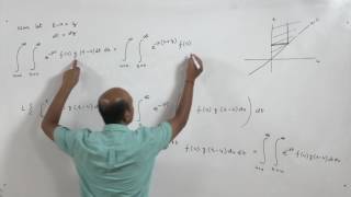
Proof Outline:
1. Use the definition of convolution.
2. Apply Laplace Transform to the convolution integral:
L{(f ∗g)(t)} = L{Z t (f(τ)g(t−τ)dτ) from 0 to t}
3. Change the order of integration (by Fubini's Theorem or substitution).
4. Evaluate the inner integral and show it equals the product F(s)·G(s).
Detailed Explanation
To prove the theorem, you start by using the definition of convolution, which integrates the product of the two functions over a specified range. Then, you apply the Laplace Transform to this integral. By switching the order of integration, which is validated by Fubini's Theorem, you focus on only one of the variables at a time. After evaluating an inner integral, you will find it simplifies to the product of the two transforms, demonstrating the theorem's validity.
Examples & Analogies
Think of the proof as baking a cake. First, you gather the ingredients (definition of convolution), then you mix them together (apply Laplace Transform). If you decide to mix the dry ingredients first separately before adding wet ingredients, it's akin to changing the order of integration. Finally, baking the cake produces an end result (the product F(s)·G(s)) that combines all your hard work into one delicious baked good!
Key Insight from the Theorem
Chapter 3 of 3
🔒 Unlock Audio Chapter
Sign up and enroll to access the full audio experience
Chapter Content
Thus, convolution in the time domain becomes multiplication in the Laplace domain.
Detailed Explanation
This insight indicates that the operation of convolution, which may seem complicated in the time domain, can be simplified to multiplication when using the Laplace Transform. This means that engineers and physicists can analyze systems more efficiently by working in the Laplace domain where multiplication is much easier to manage than integration.
Examples & Analogies
Imagine trying to combine two complex puzzles (convolution in the time domain). Once you understand the underlying relationships and tools (Laplace Transforms), you realize you can simply match pieces by color and shape (multiplication), massively speeding up the process! Instead of struggling with each piece, you can multiply your outcomes and achieve a complete puzzle much quicker.
Key Concepts
-
Convolution: The integral that defines how one function modifies the shape of another function.
-
Laplace Transform: A technique used to simplify the analysis of differential equations by moving from the time domain to the frequency domain.
-
Multiplication in the Laplace domain: The core result of the convolution theorem, indicating that the Laplace transform of a convolution is the product of individual transforms.
Examples & Applications
Example of using the convolution theorem to find the response of a system modeled by the convolution of two functions.
Application of the convolution theorem in solving complex differential equations in engineering contexts.
Memory Aids
Interactive tools to help you remember key concepts
Rhymes
Convolution's the key, simplifying for me, from time to the space where functions can play.
Stories
Imagine you are mixing two paints. The way one paint influences the color of the other is like convolution influencing one function by another.
Memory Tools
Remember: C = C(M) - Convolution Equals Convolution in the Laplace (C) domain.
Acronyms
F.C.G
Functions Combine Gently — the essence of convolution!
Flash Cards
Glossary
- Convolution
A mathematical operation that combines two functions to form a third function, describing how the shape of one is modified by the other.
- Laplace Transform
A technique for transforming a time-domain function into a complex frequency domain, simplifying the process of solving linear differential equations.
- Transform
A mathematical operation that converts one function or domain into another, such as shifting from time to frequency domain.
- Linear TimeInvariant Systems (LTI)
Systems for which superposition holds and whose characteristics do not change over time.
Reference links
Supplementary resources to enhance your learning experience.