
Method of Variation of Parameters
Enroll to start learning
You’ve not yet enrolled in this course. Please enroll for free to listen to audio lessons, classroom podcasts and take practice test.
Interactive Audio Lesson
Listen to a student-teacher conversation explaining the topic in a relatable way.
Introduction to Variation of Parameters
🔒 Unlock Audio Lesson
Sign up and enroll to listen to this audio lesson

Today, we will explore the method of variation of parameters. Can anyone tell me when we might use this method?

Is it used when the non-homogeneous term isn’t a simple polynomial or exponential?
Exactly! We resort to this method when the forcing function, f(x), doesn't fit the criteria for the method of undetermined coefficients.

So it can handle any type of f(x) then?
Correct! It’s quite powerful and versatile, though it does require integration.
Procedure of the Method
🔒 Unlock Audio Lesson
Sign up and enroll to listen to this audio lesson

Let's dive into the steps of applying this method. First, what do we do after identifying our homogeneous equation?

We solve it to find the complementary solution?
Correct! We need to find the two linearly independent solutions, y₁(x) and y₂(x). Then what do we do next?

We assume a particular integral like yₚ(x) = u₁(x)y₁(x) + u₂(x)y₂(x).
Right! Then we set up the system of equations to solve for u₁(x) and u₂(x).
Solving for u₁ and u₂
🔒 Unlock Audio Lesson
Sign up and enroll to listen to this audio lesson
After we have our equations set up, how do we solve for u₁ and u₂?
We solve the system of equations from our assumptions?
Exactly! Once we have u₁ and u₂, we integrate them to find the functions.
Then we substitute them back into our particular solution form?
That's right! The final step involves substituting and simplifying to obtain our particular integral, yₚ(x).
Introduction & Overview
Read summaries of the section's main ideas at different levels of detail.
Quick Overview
Standard
This section discusses the method of variation of parameters, outlining when and how to use it. The procedure involves solving the homogeneous equation, formulating a particular integral based on linear combinations of independent solutions, and integrating to find the specific solution that accounts for the non-homogeneity.
Detailed
Method of Variation of Parameters
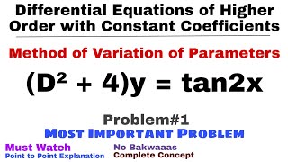
In dealing with second-order linear non-homogeneous differential equations, we often face situations where the non-homogeneous term, represented as f(x), does not fit the criteria for using the method of undetermined coefficients. In such cases, we turn to the method of variation of parameters, a versatile technique applicable for any form of f(x), despite its increased complexity due to the integration involved.
Procedure
The steps to employ the method are as follows:
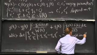
1. Identify the homogeneous equation and find its two linearly independent solutions, denoted as y₁(x) and y₂(x).
2. Assume that the particular solution has the form yₚ(x) = u₁(x)y₁(x) + u₂(x)y₂(x), where u₁(x) and u₂(x) are functions to be determined.
3. Solve the system of equations to find u₁(x) and u₂(x), and integrate them.
4. Substitute back into the assumed form to obtain yₚ(x).
This method is particularly useful in engineering applications where the forcing function can vary significantly, making it critical for accurate modeling of systems influenced by external factors.
Youtube Videos


Audio Book
Dive deep into the subject with an immersive audiobook experience.
When to Use the Method
Chapter 1 of 3
🔒 Unlock Audio Chapter
Sign up and enroll to access the full audio experience
Chapter Content
• When f(x) is not of the standard type or not suitable for undetermined coefficients.
• Works for any form of f(x), but involves integration.
Detailed Explanation
This method of variation of parameters is utilized when dealing with non-homogeneous differential equations where the forcing function, denoted f(x), does not conform to common types suitable for simpler methods like the method of undetermined coefficients. Unlike the undetermined coefficients method, which is limited to specific forms like polynomials and trigonometric functions, variation of parameters can accommodate any form of f(x). However, it requires the computation of integrals, making it a bit more complex.
Examples & Analogies
Think of it like a chef who can only use certain ingredients for a quick recipe (undetermined coefficients) but is skilled enough to use whatever is available in the kitchen (variation of parameters) to create a unique dish, knowing that it might take longer to prepare.
Procedure Overview
Chapter 2 of 3
🔒 Unlock Audio Chapter
Sign up and enroll to access the full audio experience
Chapter Content
Given:
ay′′+by′+cy =f(x)
1. Solve the homogeneous equation to find y1(x), y2(x), the two linearly independent solutions.
2. Assume:
yp(x)=u1(x)y1(x)+u2(x)y2(x)
3. Find u1(x), u2(x) by solving the system:
u1(x)y1(x)+u2(x)y2(x)=0
y1′(x)u1′(x)+y2′(x)u2′(x)=f(x)
4. Integrate u1(x), u2(x) to get u1, u2, then substitute into yp(x).
Detailed Explanation
- Solve the Homogeneous Equation: Start by solving the corresponding homogeneous equation, which allows us to determine the general behavior of the system without external forces. This gives us two linearly independent solutions, y1(x) and y2(x).
- Assume a Particular Solution: We construct a specific solution for the non-homogeneous equation in the form yp(x) = u1(x)y1(x) + u2(x)y2(x), where u1 and u2 are functions that we need to determine.
- Set Up the System: We establish a system of equations to find u1(x) and u2(x). The first equation ensures that the combination of solutions remains valid (equals zero), and the second equation relates to the original non-homogeneous function f(x).
- Integrate: Finally, we find u1 and u2 by integrating them, and in the last step, substitute back into our assumed particular solution to get the overall solution to the original equation.
Examples & Analogies
Imagine you are assembling a complex piece of furniture. First, you follow the instructions to build the basic structure (the homogeneous part). Next, you realize you want to add custom shelving and compartments (the particular solution). You make a plan for how these additions will fit into your structure, sketching out where each piece will go and how they will hold your items securely. Finally, you put everything together, ensuring each addition complements the original structure.
Example Application
Chapter 3 of 3
🔒 Unlock Audio Chapter
Sign up and enroll to access the full audio experience
Chapter Content
Solve:
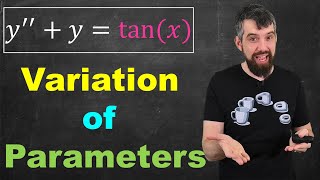
y′′+y =tanx
Solution:
• Homogeneous solution: y =C cosx + C sinx
• Let y1 = cosx, y2 = sinx
Using variation of parameters:
u1(x)cosx + u2(x)sinx = 0
−u1(x)sinx + u2(x)cosx = tanx
Solve these equations to find u1, u2, integrate, and get the particular integral.
Detailed Explanation
In this example, we want to solve the non-homogeneous equation y′′ + y = tan(x). First, we find the homogeneous solution, which is y = C1 cos(x) + C2 sin(x), where C1 and C2 are constants. Following the method of variation of parameters:
- We assume a particular solution of the form yp = u1(x) cos(x) + u2(x) sin(x).
- We form the necessary system of equations as described earlier. The first equation relates to the combination of the two function derivatives being zero, and the second equation incorporates the non-homogeneous term as tan(x).
- We then solve this system for u1 and u2, integrate, and substitute back into our assumed form to derive the particular integral for our complete solution.
Examples & Analogies
Think of it like tuning a musical instrument. At first, you have a basic melody that works (the homogeneous solution). However, as you practice more, you want to add your own unique flourish (the particular solution). You play around with different notes and harmonies (the process of solving equations) until you find the perfect fit that enhances the basic tune. Finally, you put together the original melody and your variations to create something unique and pleasing to listen to.
Key Concepts
-
Method of Variation of Parameters: A technique for solving non-homogeneous differential equations through integration of the solutions to the associated homogeneous equation.
-
Particular Solution: A specific solution that incorporates the non-homogeneous term from the differential equation.
-
Linear Independence: Essential for ensuring that the solutions to the homogeneous part do not overlap, allowing us to form a correct particular solution.
Examples & Applications
Example 1: Solve the differential equation y'' + y = tan(x) using the method of variation of parameters.
Example 2: Find the particular integral for y'' - 3y' + 2y = e^x using the method outlined in this section.
Memory Aids
Interactive tools to help you remember key concepts
Rhymes
When your f(x) won't behave, don't miss the wave, variation saves the day!
Stories
Imagine a ship (the equation) fighting against various waves (f(x)). The ship has strong sails (complementary functions) that don’t change, but the sailor (variation of parameters) must adapt the sails based on the waves to keep the ship steady.
Memory Tools
To remember steps: 'S-A-S-I' - Solve Homogeneous, Assume form, Solve for u's, Integrate!
Acronyms
To recall 'VAP' - Variation of Parameters for the non-homogeneous terms.
Flash Cards
Glossary
- NonHomogeneous Equation
A differential equation that includes a non-zero forcing function.
- Particular Integral
A specific solution to the non-homogeneous part of the differential equation.
- Complementary Function
The general solution of the corresponding homogeneous equation.
- Linear Independence
Two functions are linearly independent if no combination of them can yield zero unless both coefficients are zero.
- Homogeneous Equation
A differential equation where the non-homogeneous term is zero.
Reference links
Supplementary resources to enhance your learning experience.