
Non-Homogeneous Equations
Enroll to start learning
You’ve not yet enrolled in this course. Please enroll for free to listen to audio lessons, classroom podcasts and take practice test.
Interactive Audio Lesson
Listen to a student-teacher conversation explaining the topic in a relatable way.
Introduction to Non-Homogeneous Equations
🔒 Unlock Audio Lesson
Sign up and enroll to listen to this audio lesson

Today, we're discussing non-homogeneous differential equations that describe how systems react to external inputs or forces. Can anyone give an example of where we might encounter such equations?

How about when analyzing the deflection of a beam under a load?
Exactly! When external forces like loads are acting on a structure, we use non-homogeneous equations to model the overall response. Remember, they combine both natural and forced responses.

So, what's the general form of a non-homogeneous equation?
Great question! The general form can be expressed as d²y/dx² + b dy/dx + cy = f(x), where f(x) is the external influence. Remember this structure, as we will refer to it often.
Methods to Solve Non-Homogeneous Equations
🔒 Unlock Audio Lesson
Sign up and enroll to listen to this audio lesson

Now, let's discuss how we can actually solve these equations. There are two main methods: the method of undetermined coefficients and variation of parameters. Who has heard of either of these?

I've heard about undetermined coefficients but not the other one.
Undetermined coefficients are used when our non-homogeneous term f(x) fits a specific form. Do you remember the kinds of functions we can use?

Yes! Like polynomials or exponentials!
Precisely! If we can identify f(x) as one of those forms, we can make a guess for our particular integral. In contrast, variation of parameters works for more complex or undefined cases. Let's dig into that next!
Application in Civil Engineering
🔒 Unlock Audio Lesson
Sign up and enroll to listen to this audio lesson
Now that we've covered how to solve these equations, let’s look at their applications specifically in civil engineering. Can someone provide an example of its application?
Beam deflections and thermal conduction are both methods where we apply these equations, right?
Correct! For instance, when calculating beam deflection, the governing differential equation includes the loading conditions which are modeled as non-homogeneous terms. Understanding the response of structures under loads is crucial for safety.
What about higher-order non-homogeneous equations? How do those fit in?
Higher-order equations come into play in more complex scenarios like vibration analysis. The same fundamental methods we learned apply here, but we might faces some additional intricacies.
Special Cases: Resonance
🔒 Unlock Audio Lesson
Sign up and enroll to listen to this audio lesson
Let’s wrap up by discussing a special case: resonance. What happens when the frequency of the input matches the natural frequency of the system?
It causes an amplified response, right? That’s really important for structures!
Exactly! In our example of d²y/dx² + ω²y = cos(ωx), we need to be careful when guessing our particular integral since it matches the complementary function. We'll often multiply our guess by x to find a valid PI.
So, managing resonance is crucial in engineering designs to avoid failure?
Yes! Understanding these interactions can prevent catastrophes in civil structures. Remember this concept; it’s central in structural dynamics.
Introduction & Overview
Read summaries of the section's main ideas at different levels of detail.
Quick Overview
Standard
This section explores non-homogeneous differential equations, which arise in engineering applications due to external forces. It details the theoretical framework, methods for solving these equations, particularly the method of undetermined coefficients and variation of parameters, and their applications in civil engineering.
Detailed
Non-Homogeneous Equations
In the realm of differential equations, particularly relevant to engineering, non-homogeneous differential equations describe systems affected by external forces or inputs, such as loads on beams or heat sources in materials. Unlike homogeneous equations, which only detail a system's natural response, non-homogeneous equations account for both natural and forced responses.
General Form
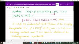
A typical second-order linear non-homogeneous differential equation with constant coefficients is given by:
where a, b, and c are constants and f(x) is the non-homogeneous term.
Solution Structure
The general solution can be written as the sum of the complementary function (CF) from the homogeneous equation and the particular integral (PI) for the non-homogeneous part.
Methods of Solution
Two principal methods for solving these equations, especially in engineering contexts, are:
-
Method of Undetermined Coefficients: This method is used when
f(x)can be expressed in a form suitable for guessing, like polynomials or exponentials. The key steps involve making an educated guess, substituting it into the original equation, and solving for coefficients. -
Method of Variation of Parameters: This applies when
f(x)does not fit the criteria for undetermined coefficients. This method involves assuming a specific form for the solution, which requires integrating functions derived from the homogeneous solutions.
Applications in Civil Engineering
Non-homogeneous equations are crucial for modeling phenomena in structural engineering, such as beam deflections under load and thermal conduction with heat sources. The ability to solve these equations allows engineers to accurately predict behavior under real-world conditions.
Higher-Order Non-Homogeneous Equations
The principles apply similarly for higher-order equations encountered in complex analyses, particularly in vibration and structural dynamics.
Special Cases: Resonance
Resonance occurs when the external forcing frequency matches a system's natural frequency, leading to amplified responses.
This chapter’s focus on non-homogeneous equations provides necessary tools for engineers to approach diverse real-world problems.
Youtube Videos


Audio Book
Dive deep into the subject with an immersive audiobook experience.
Introduction to Non-Homogeneous Equations
Chapter 1 of 13
🔒 Unlock Audio Chapter
Sign up and enroll to access the full audio experience
Chapter Content
In the study of differential equations, particularly in engineering applications, many physical systems are governed by non-homogeneous differential equations. These equations appear when external forces or inputs act on a system, such as loads on a beam, heat sources in a medium, or electrical inputs in circuits. Unlike homogeneous equations, which describe the system's natural response, non-homogeneous differential equations describe the total response, which includes both the natural and the forced responses.
Detailed Explanation
Non-homogeneous equations are crucial in engineering because they account for external influences on a system. For example, when you push down on a beam, you create a load that the beam must respond to, and the equations describing this behavior are non-homogeneous. The primary difference between homogeneous and non-homogeneous equations is that the former only looks at how a system behaves when no outside forces are applied, while the latter includes those outside forces.
Examples & Analogies
Imagine you're riding a bicycle down a hill (the natural response), but then someone nudges you to the side (the external force). The way you steer to maintain balance while going downhill represents the non-homogeneous response because it's a combination of your natural movement and the push you received.
General Form of a Linear Non-Homogeneous Differential Equation
Chapter 2 of 13
🔒 Unlock Audio Chapter
Sign up and enroll to access the full audio experience
Chapter Content
A second-order linear non-homogeneous differential equation with constant coefficients is given by:
d²y/dx² + b dy/dx + c y = f(x)
Where:
- a, b, c are constants (with a ≠ 0),
- y(x) is the unknown function,
- f(x) is a known function (non-zero), called the non-homogeneous term or forcing function.
Detailed Explanation
The general form of a linear non-homogeneous differential equation outlines how we can mathematically describe a system influenced by external forces. In this equation, 'a', 'b', and 'c' are constants that define the specific characteristics of the system, such as stiffness or resistance. The function 'f(x)' represents the external influence acting on the system, which could be anything from an applied load to a heat source.
Examples & Analogies
Think of a car moving down a road. The car's movement (denoted by 'y') is influenced by various factors: engine power (constant 'a'), friction (constant 'b'), and any bumps in the road (the function 'f(x)'). Each of these factors affects how the car responds to speed up or slow down.
General Solution Structure
Chapter 3 of 13
🔒 Unlock Audio Chapter
Sign up and enroll to access the full audio experience
Chapter Content
The general solution y(x) of the non-homogeneous equation is given by:
y(x) = y_h(x) + y_p(x)
Where:
- y_h(x) is the complementary function (CF): the general solution of the corresponding homogeneous equation:
d²y/dx² + b dy/dx + c y = 0
- y_p(x) is the particular integral (PI): a specific solution to the non-homogeneous equation.
Detailed Explanation
In solving non-homogeneous equations, we find that the total solution can be broken down into two parts: the complementary function, which captures the response of the system without external forces, and the particular integral, which accounts for those external forces. This separation helps in tackling complex problems by first understanding the system's natural behavior (homogeneous part) and then how it reacts to outside influences (particular integral).
Examples & Analogies
Consider baking a cake. The complementary function is the cake batter itself, which is a consistent foundation for every cake. The particular integral represents the icing and decorations that customize the cake for a particular occasion. Just as the icing enhances the cake, the particular integral adds the external forces to the solution.
Solving the Homogeneous Part
Chapter 4 of 13
🔒 Unlock Audio Chapter
Sign up and enroll to access the full audio experience
Chapter Content
To find y_h(x), solve the auxiliary (or characteristic) equation:
a r² + b r + c = 0
Let the roots be:
- Distinct real: r₁, r₂ → y_h = C₁ e^(r₁x) + C₂ e^(r₂x)
- Repeated real: r → y_h = (C₁ + C₂ x)e^(r₁x)
- Complex: α ± βi → y_h = e^(αx)(C₁ cos(βx) + C₂ sin(βx))
This step is identical for both homogeneous and non-homogeneous equations.
Detailed Explanation
To solve for the complementary function, we work with the characteristic equation derived from the homogeneous part of the differential equation. Based on the nature of the roots (real or complex), we apply different formulas to construct the general solution. This process is crucial because it allows us to find how the system behaves on its own, exactly the way it would without any outside influences.
Examples & Analogies
Imagine tuning a guitar. The notes you play are akin to the roots of the characteristic equation. Depending on whether you hit a perfect note (distinct real roots), a note that resonates (repeated real roots), or a note blend (complex roots), you get different sounds – just like different behaviors of a system responding to initial conditions without external forces.
Finding the Particular Integral
Chapter 5 of 13
🔒 Unlock Audio Chapter
Sign up and enroll to access the full audio experience
Chapter Content
There are multiple methods for finding y_p(x). The most common ones used in engineering applications are:
6.3.1 Method of Undetermined Coefficients
- When to Use: Only when f(x) is a linear combination of functions like:
- Polynomials (e.g. x, x²)
- Exponentials (e.g. e^ax)
- Trigonometric functions (e.g. sinx, cosx)
- Their products (e.g. xe^x, e^x cosx, etc.)
- Procedure:
- Guess a form for y_p(x), based on the form of f(x), with unknown coefficients.
- Substitute this guess into the differential equation.
- Determine the coefficients by matching both sides.
Important Note: If the guessed form for y is a solution of the homogeneous part, multiply by x or a higher power of x until linear independence is achieved.
Detailed Explanation
Finding the particular integral is an essential step to fully understand how a system reacts under external influences. The method of undetermined coefficients is often the go-to approach when the non-homogeneous term can be represented by familiar functions. The procedure involves making an educated guess, substituting it back into the equation, and solving for the coefficients to satisfy the relationship.
Examples & Analogies
Think of it like choosing an outfit for a specific occasion. If you know the event (the external force), you can pick clothes (the form of y_p(x)) that match. If you choose something too similar to what you usually wear (a solution of the homogeneous part), you might need to modify it (multiply by x) to ensure it stands out appropriately for the event.
Method of Variation of Parameters
Chapter 6 of 13
🔒 Unlock Audio Chapter
Sign up and enroll to access the full audio experience
Chapter Content
When to Use:
- When f(x) is not of the standard type or not suitable for undetermined coefficients.
- Works for any form of f(x), but involves integration.
Procedure Given:
- a y'' + b y' + c y = f(x)
1. Solve the homogeneous equation to find y₁(x), y₂(x), the two linearly independent solutions.
2. Assume:
y_p(x) = u₁(x) y₁(x) + u₂(x) y₂(x)
3. Find u₁(x), u₂(x) by solving the system:
u₁'(x) y₁(x) + u₂'(x) y₂(x) = 0
-u₁'(x) y₁'(x) + u₂'(x) y₂'(x) = f(x)
4. Integrate u₁(x), u₂(x) to get u₁, u₂, then substitute into y_p(x).
Detailed Explanation
The variation of parameters is a more flexible method for finding the particular integral, especially when the non-homogeneous term doesn't fit neatly into the forms suitable for the undetermined coefficients method. It involves using the solutions from the homogeneous equation to construct a new function, where the coefficients are allowed to vary instead of being constant. This provides a way to account for a wider range of external influences.
Examples & Analogies
Imagine if you were trying to cook a dish but the recipe didn't align with the ingredients you have at home. Instead of sticking to the recipe, you adapt by using what you have (the solutions to the homogeneous equation) and varying the amounts as needed to make something delicious (the particular integral).
Applications in Civil Engineering
Chapter 7 of 13
🔒 Unlock Audio Chapter
Sign up and enroll to access the full audio experience
Chapter Content
Non-homogeneous equations are vital in:
- Beam deflection under load: Governing differential equation:
d⁴y/dx⁴ = w(x)/EI
where w(x) is the distributed load (forcing function).
- Thermal conduction with sources:
d²T/dx² = -q(x)/k
where q(x) is the heat source.
- Fluid flow problems where external forces like pressure or gravity act on the system.
Being able to solve non-homogeneous equations equips civil engineers to model and analyze these physical systems accurately.
Detailed Explanation
In civil engineering, non-homogeneous equations are used extensively to model real-world scenarios where external forces affect structural behavior. This includes analyzing how beams bend under loads, tracking heat distributed in a medium, or observing how fluids move under varying pressures. By solving these equations, engineers can create accurate models for design and safety.
Examples & Analogies
Think of a bridge: when vehicles drive over it, the weight they apply is an external force that affects how the bridge bends and moves. This bending can be predicted using non-homogeneous equations that help engineers ensure that bridges are safely constructed to withstand the loads they encounter.
Higher-Order Non-Homogeneous Equations
Chapter 8 of 13
🔒 Unlock Audio Chapter
Sign up and enroll to access the full audio experience
Chapter Content
In civil engineering applications, sometimes third-order or fourth-order non-homogeneous equations occur, especially in beam theory and vibration analysis. A general nth-order linear non-homogeneous differential equation:
dⁿy/dxⁿ + a₁dⁿ⁻¹y/dxⁿ⁻¹ + ... + aₙy = f(x)
Solution Methodology:
1. Find the Complementary Function (CF) by solving the homogeneous equation.
2. Use the method of undetermined coefficients or variation of parameters to find the particular integral (PI).
3. Combine both for the general solution:
y(x) = y_h(x) + y_p(x)
Detailed Explanation
Higher-order non-homogeneous equations extend the principles we discussed earlier to more complex systems where multiple factors influence the behavior of a structure. The methodology remains consistent: find the complementary function from the homogeneous part and then determine the particular integral based on the external forces. Combining these solutions allows for a complete understanding of the system's response.
Examples & Analogies
Imagine a concert hall. The sound produced by a single instrument is like the response of a second-order system. But when multiple instruments play together (a higher-order system), you need to understand how each contributes to the overall sound, requiring a more complex analysis similar to how we handle higher-order equations.
Special Case: Resonance
Chapter 9 of 13
🔒 Unlock Audio Chapter
Sign up and enroll to access the full audio experience
Chapter Content
In mechanical and structural systems, resonance occurs when the frequency of the forcing function matches the natural frequency of the system.
Example of Resonance:
Consider:
d²y/dx² + ω²y = cos(ωx)
Here, the forcing function cos(ωx) matches the natural frequency of the system.
Solution Approach:
1. CF: y = C cos(ωx) + C sin(ωx)
2. Since cos(ωx) appears in the CF, guessing PI as A cos(ωx) + B sin(ωx) fails.
Modification Rule: Multiply the guess by x → Try:
y = x(A cos(ωx) + B sin(ωx))
Detailed Explanation
Resonance is a significant phenomenon in mechanical systems where the input frequency aligns with the natural frequency of the system, leading to amplified responses. In mathematical terms, if we naively try to guess a particular integral that is similar to the complementary function, it won't work because it already forms part of the solution. Instead, we modify our guess to represent this larger response, acknowledging how the system will behave under resonant conditions.
Examples & Analogies
Think of pushing someone on a swing. If you push in sync with the swing's natural rhythm (resonance), the swing goes higher and higher. However, if you push at a different rhythm, you'd get less effect. The swing embodies the principles of resonance where the energy builds up effectively when synchronized.
Non-Homogeneous Systems of Differential Equations
Chapter 10 of 13
🔒 Unlock Audio Chapter
Sign up and enroll to access the full audio experience
Chapter Content
Civil engineering models often involve multiple dependent variables interacting. For instance:
dx/dt = 3x + 4y + sin(t)
dy/dt = -4x + 3y + e^t
This system is non-homogeneous due to the sine and exponential terms.
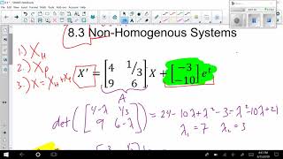
Solution Outline:
1. Solve the homogeneous system using eigenvalues/eigenvectors.
2. Use variation of parameters or an integrating factor matrix to find the particular solution.
Detailed Explanation
When multiple variables interact, we end up with a system of differential equations that may not be homogeneous due to the presence of specific functions like sine and exponentials. To solve these systems, we typically begin with the homogeneous part and then incorporate the effects of the non-homogeneous terms using methods like variation of parameters, which allows us to find a solution that accurately describes the system's behavior.
Examples & Analogies
Consider a traffic system where the flow of cars (x) and pedestrians (y) influence each other. If a traffic light changes (external factor), it affects both the cars and pedestrians. We can model this interaction with differential equations that reflect how each group influences the other, much like how we solve for dependent variables in our equations.
Worked Examples with Engineering Applications
Chapter 11 of 13
🔒 Unlock Audio Chapter
Sign up and enroll to access the full audio experience
Chapter Content
Example 1: Beam Under Uniform Load
Given:
d⁴y/dx⁴ = q
Where:
- EI = flexural rigidity of the beam
- q = uniform load per unit length
Solution:
Rewriting:
d⁴y/dx⁴ = 0
Integrating four times:
d³y/dx³ = (q/EI)x + C₁
d²y/dx² = (q/2EI)x² + C₁x + C₂
dy/dx = (q/6EI)x³ + (C₁/2)x² + C₂x + C₃
y(x) = (q/24EI)x⁴ + (C₁/6)x³ + (C₂/2)x² + C₃x + C₄
Boundary conditions (e.g., at fixed ends) are used to determine C₁ to C₄.
Detailed Explanation
In engineering, practical problems often require us to apply theoretical methods to real-world scenarios, such as calculating the deflection of a beam under uniform load. By setting up the governing equation and incorporating boundary conditions, we can find specific solutions that will guide how the beam should be designed to ensure safety and effectiveness under load.
Examples & Analogies
Think about how a bridge is built. Engineers calculate how much weight the structure can handle by considering the loads on the bridge (like cars) similar to how we analyze beams under loads. This ensures the bridge can support its intended traffic flow without collapsing.
Vibration of a Damped System with Forcing
Chapter 12 of 13
🔒 Unlock Audio Chapter
Sign up and enroll to access the full audio experience
Chapter Content
Given:
d²y/dt² + c dy/dt + k y = F cos(ωt)
This is a non-homogeneous second-order ODE representing a damped forced vibration.
- Solve the homogeneous equation:
mr² + cr + k = 0
- Based on discriminant, determine y_h
- Guess PI using undetermined coefficients (if ω ≠ ω₀) or resonance form (if ω = ω₀).
Detailed Explanation
When analyzing vibrations in structures, we often encounter damped systems that include external forces. The approach involves finding the homogeneous solution first, then determining the particular integral based on whether the frequency of the driving force resonates with the natural frequency of the system. By evaluating these aspects, we can predict how the structure will perform under vibrations.
Examples & Analogies
Imagine a suspension bridge swaying due to wind or traffic – the vibrations are akin to the damping and forcing described in the equation. By understanding these vibrations, we can ensure the bridge remains stable and responsive, much like tuning a musical instrument to achieve the perfect sound.
Conceptual Notes
Chapter 13 of 13
🔒 Unlock Audio Chapter
Sign up and enroll to access the full audio experience
Chapter Content
• Non-homogeneous differential equations model forced systems — very common in civil structures where loads, vibrations, or heat sources exist.
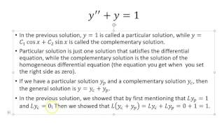
• If the forcing function f(x) is zero → the equation becomes homogeneous, representing free vibration or natural behavior.
• The method of undetermined coefficients is easier but limited.
• The method of variation of parameters is powerful and general, but involves more calculation.
Detailed Explanation
It's essential to grasp the overall concepts surrounding non-homogeneous equations and their applications in engineering. These equations allow engineers to model and analyze systems influenced by outside forces. Understanding when to apply each method is crucial – while the method of undetermined coefficients is simpler, the method of variation of parameters provides more flexibility for a wider range of problems.
Examples & Analogies
Think of planning a big event. If the event goes as expected, you will have a simpler setup (homogeneous). But when guests bring unexpected items or changes happen, you have to adapt (non-homogeneous). Using simpler plans is great, but sometimes you have to dive deeper with more detailed backup plans – that’s how these methods apply to solving real-life engineering challenges.
Key Concepts
-
General Form: The standard structure of a non-homogeneous equation.
-
Complementary Function: The natural response of the system from the homogeneous part.
-
Particular Integral: The specific solution that accounts for the external influences.
-
Method of Undetermined Coefficients: A method suitable for certain functional forms of f(x).
-
Variation of Parameters: A versatile method applicable to all f(x) forms.
-
Resonance: A critical behavior to manage in engineering to avoid structural failure.
Examples & Applications
Example of solving d²y/dx² - 3 dy/dx + 2y = e^x using the method of undetermined coefficients.
Illustration of resonance through the equation d²y/dx² + ω²y = cos(ωx).
Memory Aids
Interactive tools to help you remember key concepts
Rhymes
When forces act on beams or heat flows too, / Non-homogeneous equations help engineers see what's true.
Stories
Imagine a bridge that shakes when trucks go across. This resonance can lead to disaster, but engineers now know how to calculate and prevent that chaos.
Memory Tools
RAP: Resonance Amplifies Problems in structures when frequencies align.
Acronyms
CFR
Complementary Function + Forcing Response = Non-Homogeneous.
Flash Cards
Glossary
- NonHomogeneous Differential Equation
A differential equation that includes terms representing external forces or influences, leading to a total response that combines natural and forced responses.
- Complementary Function (CF)
The solution to the homogeneous part of the differential equation, representing the system's natural response.
- Particular Integral (PI)
A specific solution to the non-homogeneous equation that accounts for the system's response due to external forces.
- Method of Undetermined Coefficients
A technique for finding particular solutions of non-homogeneous equations when the forcing term fits specific functional forms.
- Method of Variation of Parameters
A method for finding particular solutions for non-homogeneous equations appropriate for situations where the forcing term is more complex.
- Resonance
A phenomenon where the frequency of an external force matches a system's natural frequency, leading to amplified oscillations or responses.
Reference links
Supplementary resources to enhance your learning experience.