
Solving the Homogeneous Part
Enroll to start learning
You’ve not yet enrolled in this course. Please enroll for free to listen to audio lessons, classroom podcasts and take practice test.
Interactive Audio Lesson
Listen to a student-teacher conversation explaining the topic in a relatable way.
Introduction to the Homogeneous Part
🔒 Unlock Audio Lesson
Sign up and enroll to listen to this audio lesson

Let’s start by discussing the importance of solving the homogeneous part of a differential equation. What do you understand by a homogeneous equation?

I think it's an equation where non-homogeneous terms are absent.
Correct, well done! This means it only deals with terms involving the unknown variable and its derivatives. Let's dive into the auxiliary equation used for these kinds of equations.
The Characteristic Equation
🔒 Unlock Audio Lesson
Sign up and enroll to listen to this audio lesson

To find the complementary function, we solve the auxiliary equation which is derived from the homogeneous equation. What is the general form of this equation?

Is it ar² + br + c = 0?
Exactly! Once we solve for the roots, they guide us in forming the complementary function. Can anyone tell me what happens if we get distinct real roots?

We use the form \(y_h = C_1 e^{r_1 x} + C_2 e^{r_2 x}\)!
Great! This will leverage our understanding of the solutions. Now, what about repeated roots?

For repeated roots, it becomes \(y_h = (C_1 + C_2 x)e^{r x}\)!
Exactly! That’s the unique aspect of such roots.
Complex Roots
🔒 Unlock Audio Lesson
Sign up and enroll to listen to this audio lesson
Now, let’s consider what we do when we encounter complex roots. Can someone explain how we express the complementary function?
For complex roots, I think we use the form \(y_h = e^{αx}(C_1 cos(βx) + C_2 sin(βx))\)!
Excellent! The exponential decay/growth factor represented by the \(α\) term modulates the oscillatory behavior dictated by the \(β\) term. It plays a crucial role in physical systems modeled by these equations!
Synthesis and Application
🔒 Unlock Audio Lesson
Sign up and enroll to listen to this audio lesson
Let’s summarize the significance of solving the homogeneous part before applying it to real-world problems. Why is this step critical?
Because it forms the foundation for solving the entire differential equation!
Absolutely! Understanding the behavior of the system without external inputs must come first. Before we move on to finding particular solutions, does anyone think of a real-life application of these equations?
Maybe in building structural analysis?
Or in electrical circuits too!
Both excellent examples! These equations model foundational behaviors crucial for civil engineers.
Introduction & Overview
Read summaries of the section's main ideas at different levels of detail.
Quick Overview
Standard
The section discusses the process of solving the homogeneous part of a non-homogeneous differential equation by determining the roots of the auxiliary equation. Based on the nature of the roots (distinct, repeated, or complex), different forms of the complementary function are constructed to arrive at the solution.
Detailed
Detailed Summary
In differential equations, particularly when dealing with non-homogeneous equations, it is crucial first to solve the homogeneous part. This section highlights:
- The Auxiliary (Characteristic) Equation: This foundational step involves writing down the characteristic polynomial for the homogeneous equation and determining its roots.
- The general second-order homogeneous equation takes the form: $$a r^2 + b r + c = 0$$
- Roots of the Auxiliary Equation: The roots lead to different forms for the complementary function (CF), defined as follows:
- Distinct Real Roots: If the roots are distinct and real (\(r_1, r_2\)), the solution takes the form:
$$y_h = C_1 e^{r_1 x} + C_2 e^{r_2 x}$$ - Repeated Real Roots: If the roots are repeated (\(r\)), the solution is:
$$y_h = (C_1 + C_2 x) e^{r x}$$ - Complex Roots: For complex roots (\(α ± βi\)), the solution is:
$$y_h = e^{αx}(C_1 ext{cos}(β x) + C_2 ext{sin}(β x))$$
This system of solving for the homogeneous part is crucial because it sets the stage for determining the particular solution of the non-homogeneous differential equation in subsequent sections.
Youtube Videos


Audio Book
Dive deep into the subject with an immersive audiobook experience.
Finding the Complementary Function
Chapter 1 of 3
🔒 Unlock Audio Chapter
Sign up and enroll to access the full audio experience
Chapter Content
To find y (x), solve the auxiliary (or characteristic) equation:
har² + br + c = 0
Detailed Explanation
To begin solving the homogeneous part of a differential equation, we first need to find the complementary function, denoted as yh(x). This involves solving the characteristic equation derived from the polynomial formed by substituting derivatives into the differential equation. Specifically, we set up the equation ar² + br + c = 0, where a, b, and c are constants, and we solve this quadratic equation for its roots. The roots can be real and distinct, real and repeated, or complex.
Examples & Analogies
Think of the process like finding the roots of a plant. Just as the health of a plant depends on the strength and spread of its roots below the surface, the behavior of a physical system (like a beam under load) depends on the roots derived from the characteristic equation. Each type of root tells us a different aspect of the system's response.
Types of Roots and Their Solutions
Chapter 2 of 3
🔒 Unlock Audio Chapter
Sign up and enroll to access the full audio experience
Chapter Content
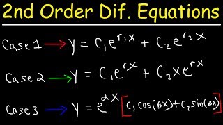
Let the roots be:
• Distinct real: r1, r2 → yh = C1e^(r1x) + C2e^(r2x)
• Repeated real: r → yh = (C1 + C2x)e^(r1x)
• Complex: α±βi → yh = e^(αx)(C1 cos(βx) + C2 sin(βx))
Detailed Explanation
Once we find the roots of the characteristic equation, the nature of these roots determines the form of our complementary function, yh(x). If we have two distinct real roots, we express the solution as a linear combination of exponentials. In cases of repeated roots, we introduce an additional x term to maintain independence in the solutions. For complex roots, we use Euler's formula, expressing the solution in terms of sine and cosine functions, which represent oscillatory behaviors.
Examples & Analogies
Imagine you are tuning an instrument. Distinct real roots are like two different notes played together that sound harmonious. When the roots are repeated, it’s akin to playing the same note at a different pitch, creating depth. Lastly, complex roots relate to vibrations, like a guitar string that oscillates back and forth — this oscillation is represented mathematically with sine and cosine.
Identical Steps for Homogeneous and Non-Homogeneous Equations
Chapter 3 of 3
🔒 Unlock Audio Chapter
Sign up and enroll to access the full audio experience
Chapter Content
This step is identical for both homogeneous and non-homogeneous equations.
Detailed Explanation
A key point to remember is that the process of solving for the complementary function is the same regardless of whether we are dealing with a homogeneous or a non-homogeneous differential equation. The foundational work of finding the roots and establishing yh(x) remains consistent because both types of equations still rely on the underlying characteristics of their differential structure.
Examples & Analogies
Consider a recipe for making bread. The initial steps — mixing ingredients and kneading the dough — are the same whether you’re making regular bread or adding toppings like fruit or nuts. Just as both types of bread start from the same base recipe, homogeneous and non-homogeneous equations share the same approach for finding their complementary solution.
Key Concepts
-
Auxiliary Equation: The equation derived for a homogeneous differential equation to find roots.
-
Complementary Function: The solution that corresponds to the roots of the auxiliary equation.
-
Roots Types: Distinct, repeated, and complex roots dictate the form of the complementary function.
Examples & Applications
For the equation \(d^2y/dx^2 - 3dy/dx + 2y = 0\): The auxiliary equation is \(r^2 - 3r + 2 = 0\) yielding distinct real roots 1 and 2. The complementary function is \(y_h = C_1 e^x + C_2 e^{2x}\).
If we consider repeated roots with \(d^2y/dx^2 - 4dy/dx + 4y = 0\), the roots are 2, 2. Therefore, the complementary function becomes \(y_h = (C_1 + C_2 x)e^{2x}\).
Memory Aids
Interactive tools to help you remember key concepts
Rhymes
If roots are distinct, you see,
Stories
Imagine a plant growing up, with two branches representing distinct roots; they start at the ground and grow tall under the sun, each reaching for brightness in the differential equation.
Memory Tools
For roots: RD = Real Distinct, RL = Real Repeated, CC = Complex Conjugate; Just remember the three amigos!
Acronyms
DRC - Distinct, Repeated, Complex; it stands for the types of roots impacting the solutions.
Flash Cards
Glossary
- Homogeneous Equation
An equation where the non-homogeneous terms are zero or absent.
- Auxiliary Equation
A characteristic polynomial derived from a differential equation, used to find the roots.
- Complementary Function (CF)
The general solution of a corresponding homogeneous equation.
- Particular Integral (PI)
A specific solution to a non-homogeneous differential equation.
- Distinct Real Roots
Roots which are different and exist on the real number line.
- Repeated Real Roots
Roots that are the same and correspond to a single root in the characteristic equation.
- Complex Roots
Roots that involve imaginary numbers, typically appearing as conjugate pairs.
Reference links
Supplementary resources to enhance your learning experience.