
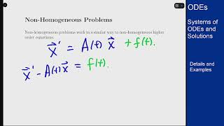
Non-Homogeneous Systems of Differential Equations
Enroll to start learning
You’ve not yet enrolled in this course. Please enroll for free to listen to audio lessons, classroom podcasts and take practice test.
Interactive Audio Lesson
Listen to a student-teacher conversation explaining the topic in a relatable way.
Introduction to Non-Homogeneous Systems
🔒 Unlock Audio Lesson
Sign up and enroll to listen to this audio lesson

Today, we will discuss non-homogeneous systems of differential equations, which are crucial in modeling complex engineering scenarios. Can anyone explain what 'non-homogeneous' means in this context?

I think it means that there are external factors or inputs affecting the system, unlike in a homogeneous system where only the system's natural behavior matters.
Exactly! Non-homogeneous equations describe the overall response, reflecting both natural behavior and forced influences. Does anyone have examples where we might see this?

Yes! One example is when modeling a beam with an applied load.
Great! Now let’s dive into a specific non-homogeneous system.
Analyzing a Non-Homogeneous System
🔒 Unlock Audio Lesson
Sign up and enroll to listen to this audio lesson

Let’s analyze the following system: $$\frac{dx}{dt} = 3x + 4y + \sin(t)$$ and $$\frac{dy}{dt} = -4x + 3y + e^t$$. Who can identify the non-homogeneous components?

The $\sin(t)$ and $e^t$ terms make it non-homogeneous.
Exactly! These terms act as external forces. Now, how would we approach solving this system?

We first find the homogeneous solution using eigenvalues and eigenvectors, right?
Correct! Solving the homogeneous part gives us an understanding of the system’s natural behavior. Let’s remember: **Eigenvalues indicate stability** and **Eigenvectors describe modes of motion**.
Finding Particular Solutions
🔒 Unlock Audio Lesson
Sign up and enroll to listen to this audio lesson
Once we have the homogeneous part, we need to find the particular solution. What methods can we use?
We could use variation of parameters or an integrating factor matrix, right?
Exactly! Variation of parameters is often more flexible but requires integration. Remember, **variation of parameters = flexible method**. Can anyone explain how we apply it?
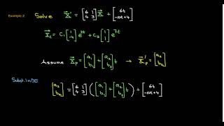
We assume a particular solution based on the form of the non-homogeneous term and solve for the coefficients!
Correct! In the context of civil engineering, understanding how to derive particular solutions can significantly improve our model accuracy.
Application in Civil Engineering
🔒 Unlock Audio Lesson
Sign up and enroll to listen to this audio lesson
Let’s discuss some applications of non-homogeneous systems in civil engineering. How do these equations help us model physical scenarios?
They help us account for things like external loads on beams or fluid dynamics with pressure changes.
Exactly! By applying these methods, engineers can predict system responses, ensuring structures are designed safely. Let's wrap up our session by summarizing key points.
So we learned about the definitions, how to analyze a non-homogeneous system, and the significance of finding particular solutions.
Great recap! Always remember that **understanding interactions between variables is essential** in civil engineering.
Introduction & Overview
Read summaries of the section's main ideas at different levels of detail.
Quick Overview
Standard
In this section, we explore non-homogeneous systems of differential equations that frequently appear in civil engineering. The section illustrates how external forces affect systems characterized by multiple interacting variables and outlines a solution approach that involves determining common eigenvalues, eigenvectors, and utilizing variation of parameters or integrating factor matrices.
Detailed
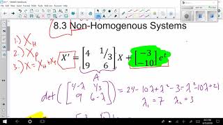
Non-Homogeneous Systems of Differential Equations
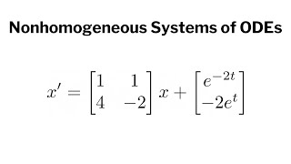
In civil engineering, physical models often consist of multiple interacting dependent variables. For example, consider the following non-homogeneous system:
$$\frac{dx}{dt} = 3x + 4y + \sin(t)$$
$$\frac{dy}{dt} = -4x + 3y + e^t$$
Here, the terms $\sin(t)$ and $e^t$ indicate the presence of external forces, rendering the system non-homogeneous.
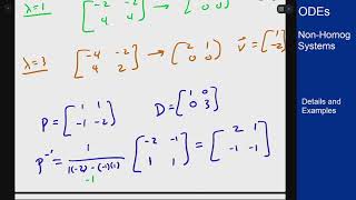
To solve this system, the first step involves solving the homogeneous system, usually achieved through eigenvalues and eigenvectors, which characterize the system's natural behavior. The subsequent step entails applying methods such as variation of parameters or using an integrating factor matrix to find the particular solution.
In summary, the approach to solving non-homogeneous systems bridges into matrix methods and Laplace transforms that will be explored in upcoming chapters, demonstrating the complexity and interdependence of engineering systems.
Youtube Videos


Audio Book
Dive deep into the subject with an immersive audiobook experience.
Introduction to Non-Homogeneous Systems
Chapter 1 of 3
🔒 Unlock Audio Chapter
Sign up and enroll to access the full audio experience
Chapter Content
Civil engineering models often involve multiple dependent variables interacting. For instance:
$$\frac{dx}{dt} = 3x + 4y + \sin(t)$$
$$\frac{dy}{dt} = -4x + 3y + e^t$$
This system is non-homogeneous due to the sine and exponential terms.
Detailed Explanation
In civil engineering, systems often involve different variables that depend on one another. For example, you might have two variables, x and y, that change over time (t). The equations provided show how the rate of change of x and y is influenced by their current values and some external forces (like the sine and exponential functions). These additional terms make the system non-homogeneous, which means it’s influenced by forces outside of the natural behavior of the system itself.
Examples & Analogies
Imagine you're a civil engineer designing a bridge. The stress on the bridge (x) not only depends on its own weight but also on factors like wind (sin(t)) and temperature changes (e^t). Just as these environmental factors change how the bridge responds, the terms in our equations do the same for the variables x and y.
Solution Outline for Non-Homogeneous Systems
Chapter 2 of 3
🔒 Unlock Audio Chapter
Sign up and enroll to access the full audio experience
Chapter Content
• Solve the homogeneous system using eigenvalues/eigenvectors.
• Use variation of parameters or an integrating factor matrix to find the particular solution.
Detailed Explanation
To solve a non-homogeneous system of differential equations, we first address the homogeneous part. This means we solve for the system without the influence of external forces. We typically use techniques such as eigenvalues and eigenvectors for this. Once we have the homogeneous solution, we then look for a particular solution that accounts for the external factors, often using methods like variation of parameters or integrating factor matrices.
Examples & Analogies
Going back to our bridge example, first, we'd analyze how the bridge would behave just under its own weight (the homogeneous system). After understanding this basic behavior, we would then factor in how things like wind and temperature affect it (the non-homogeneous terms) to get a complete picture of the bridge's performance under real-world conditions.
Transition to Advanced Methods
Chapter 3 of 3
🔒 Unlock Audio Chapter
Sign up and enroll to access the full audio experience
Chapter Content
This topic bridges into matrix methods and Laplace transforms, introduced in later chapters.
Detailed Explanation
The techniques learned for solving non-homogeneous systems set the groundwork for more advanced methods in later studies. Matrix methods will allow us to handle larger systems of equations more efficiently, while Laplace transforms provide a powerful tool for transforming and solving differential equations, particularly in the context of initial value problems.
Examples & Analogies
Consider learning to navigate a city. First, you learn the basic streets and landmarks (like the methods to solve simple systems). As you gain experience, you learn to read maps and use GPS efficiently to navigate complex road systems (like moving to matrix methods and Laplace transforms). This is how we progress from simple to complex problem-solving in engineering!
Key Concepts
-
Non-Homogeneous Systems: Systems affected by external forces or terms making them non-homogeneous.
-
Eigenvalues & Eigenvectors: Fundamental concepts for analyzing system behavior in dynamics.
-
Particular Solutions: Specific solutions that accommodate the effects of external forces.
Examples & Applications
Example of a non-homogeneous system: $$\frac{dx}{dt} = 3x + 4y + \sin(t); \frac{dy}{dt} = -4x + 3y + e^t$$
Application in beam deflection and fluid dynamics in response to external loads.
Memory Aids
Interactive tools to help you remember key concepts
Rhymes
To solve with ease, eigenvalues please, they show stability like sturdy trees.
Stories
Imagine engineers grappling with waves of data, hunting down eigenvalues to bring stability to their structural dreams.
Memory Tools
E for Eigenvalues, P for Particular solutions, remember EP for essential concepts.
Acronyms
NSES
Non-homogeneous Systems having External forces.
Flash Cards
Glossary
- NonHomogeneous Equation
A differential equation that includes external forces or inputs affecting the system.
- Eigenvalues
Values that help determine the stability and behavior of a dynamic system.
- Eigenvectors
Vectors that define the direction of system response corresponding to eigenvalues.
- Particular Solution
A specific solution to a non-homogeneous differential equation, addressing forced inputs.
- Variation of Parameters
A method used to find particular solutions for non-homogeneous differential equations.
Reference links
Supplementary resources to enhance your learning experience.