
Canonical (Standard) Forms of Second-Order PDEs
Enroll to start learning
You’ve not yet enrolled in this course. Please enroll for free to listen to audio lessons, classroom podcasts and take practice test.
Interactive Audio Lesson
Listen to a student-teacher conversation explaining the topic in a relatable way.
Introduction to Second-Order PDEs
🔒 Unlock Audio Lesson
Sign up and enroll to listen to this audio lesson

Today, we are going to explore how to transform second-order partial differential equations into their canonical forms.

What do we mean by a second-order PDE?
Great question! A second-order PDE involves second-order partial derivatives. For example, we can express it as \( A \frac{\partial^2 u}{\partial x^2} + B \frac{\partial^2 u}{\partial x \partial y} + C \frac{\partial^2 u}{\partial y^2} + \text{lower order terms} = 0 \).

What roles do A, B, and C play?
They are coefficients that can influence the equation's classification. Now, let's remember the mnemonic 'ABC - Always Builds Character' for coefficients A, B, and C.
Canonical Forms and Their Importance
🔒 Unlock Audio Lesson
Sign up and enroll to listen to this audio lesson

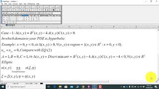
Once we express the PDE in canonical form, we can solve it more easily. The canonical forms are: the elliptic form, \( \frac{\partial^2 u}{\partial \xi^2} + \frac{\partial^2 u}{\partial \eta^2} = 0 \), the parabolic form, \( \frac{\partial^2 u}{\partial \xi^2} = \frac{\partial u}{\partial \eta} \), and the hyperbolic form, \( \frac{\partial^2 u}{\partial \xi \partial \eta} = 0 \).

Can you explain how we determine which form it takes?
Certainly! We gauge this by using the discriminant \( D = B^2 - 4AC \).

Are there specific applications where each form is used?
Yes, they are often tied to specific physical phenomena, like heat conduction or wave propagation.
Change of Variables
🔒 Unlock Audio Lesson
Sign up and enroll to listen to this audio lesson
To transition to canonical forms, we employ a change of variables, typically defining new variables \( \xi \) and \( \eta \) based on our original variables x and y.
What does this change accomplish?
It allows us to simplify the equation so that we can analyze it more efficiently.
Could you give an example of such a transformation?
Certainly! Suppose we want to transform an elliptic PDE; you might set \( \xi = x + y \) and \( \eta = x - y \).
Discussion on Discriminant
🔒 Unlock Audio Lesson
Sign up and enroll to listen to this audio lesson
The discriminant \( D\) is pivotal in determining the form of our PDE, indicated by its sign.
So, if D is negative, we have an elliptic equation?
Exactly! And if D is zero, we get a parabolic equation, while a positive D indicates a hyperbolic equation.
What’s the significance of knowing these classifications?
It influences the approach we take for finding solutions in practical applications, especially in engineering.
Summary of Canonical Forms
🔒 Unlock Audio Lesson
Sign up and enroll to listen to this audio lesson
To summarize, we've learned how to rewrite second-order PDEs into canonical forms.
What are those forms again?
We classified them into elliptic, parabolic, and hyperbolic based on the discriminant. Remember the phrase 'D Determines Definition!' to keep that in mind!
Can we apply these forms in real-world problems?
Absolutely! Engineers apply these concepts to model phenomena in structural analysis, fluid dynamics, and thermal interactions.
Introduction & Overview
Read summaries of the section's main ideas at different levels of detail.
Quick Overview
Standard
The transformation of second-order PDEs into their canonical forms is essential in simplifying their solutions. This section outlines the general form of a second-order PDE, the method to achieve canonical forms via variable change, and the classification of PDEs based on their discriminant.
Detailed
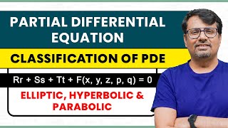
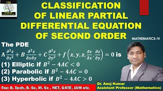
In this section, we focus on the process of transforming second-order partial differential equations (PDEs) into their canonical forms to simplify solving them analytically. A general second-order PDE in two variables can be expressed as:
$$ A \frac{\partial^2 u}{\partial x^2} + B \frac{\partial^2 u}{\partial x \partial y} + C \frac{\partial^2 u}{\partial y^2} + \text{lower order terms} = 0 $$
To facilitate solving these equations, we perform a change of variables to new variables \( \xi \) and \( \eta \) that make the equation take on one of the canonical forms.
The forms are:
- Elliptic: \( \frac{\partial^2 u}{\partial \xi^2} + \frac{\partial^2 u}{\partial \eta^2} = 0 \)
- Parabolic: \( \frac{\partial^2 u}{\partial \xi^2} = \frac{\partial u}{\partial \eta} \)
- Hyperbolic: \( \frac{\partial^2 u}{\partial \xi \partial \eta} = 0 \)
This classification depends on the discriminant \( D = B^2 - 4AC \); where the sign of D determines the type of PDE and consequently the nature of the solution. This section is crucial as it sets up the groundwork necessary for applying various methods of solving PDEs encountered in practical engineering problems.
Youtube Videos

Audio Book
Dive deep into the subject with an immersive audiobook experience.
Introduction to Canonical Forms
Chapter 1 of 7
🔒 Unlock Audio Chapter
Sign up and enroll to access the full audio experience
Chapter Content
Transforming a second-order PDE into its canonical form makes it easier to solve analytically.
Detailed Explanation
The process of transforming a second-order PDE into its canonical form is important because it simplifies the equation, making it more manageable and often easier to find solutions. Canonical forms are standard representations that emphasize the equation's properties, allowing engineers and mathematicians to apply powerful solution techniques.
Examples & Analogies
Think of this transformation like putting on a uniform for a sports team. Just as a team wears a specific uniform to identify themselves and play better together, a PDE dressed in its canonical form helps mathematicians identify the best strategies for 'playing' with their equations, leading to clearer solutions.
General Form of a Second-Order PDE
Chapter 2 of 7
🔒 Unlock Audio Chapter
Sign up and enroll to access the full audio experience
Chapter Content
Consider a general second-order PDE in two variables:
∂²u + A∂²u + B∂u + C + lower order terms = 0
∂x² ∂x∂y ∂y²
Detailed Explanation
This equation represents the general structure of a second-order partial differential equation involving two variables, where A, B, C are coefficients and may depend on the variables. The terms with second derivatives (∂²u/∂x², etc.) signify the order and type of changes we are considering in the function u, which depends on x and y.
Examples & Analogies
Imagine you're studying the height of water in a tank (the variable u) based on different levels of input (x and y). The equation captures how the water level changes not just due to direct inflow, but also due to the shape of the tank (the coefficients A, B, C).
Transforming Variables
Chapter 3 of 7
🔒 Unlock Audio Chapter
Sign up and enroll to access the full audio experience
Chapter Content
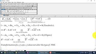
To simplify, we use a change of variables: Let ξ = ξ(x,y), η = η(x,y)
Detailed Explanation
By changing the variables from (x, y) to new variables (ξ, η), we can make the PDE simpler. The goal is to choose ξ and η so that the PDE takes on a more manageable form, which can be classified as elliptic, parabolic, or hyperbolic depending on the nature of the equation and the physical phenomena it represents.
Examples & Analogies
Consider changing the variable in an algebraic problem to make it easier to solve; like converting a complicated fraction into a more straightforward form. Similarly, these new variables help elucidate the essence of the problem and facilitate solving it.
Elliptic PDEs
Chapter 4 of 7
🔒 Unlock Audio Chapter
Sign up and enroll to access the full audio experience
Chapter Content
Elliptic: ∂²u/∂ξ² + ∂²u/∂η² = 0
Detailed Explanation
When the second-order PDE is in elliptic form, it often indicates steady-state solutions, which do not change over time. This is crucial in many applications like heat distribution where the system has reached equilibrium and is no longer changing.
Examples & Analogies
Think of it as a calm lake on a windless day. The surface remains still (just like the solution to an elliptic PDE), representing a state of equilibrium where no external forces are acting on it.
Parabolic PDEs
Chapter 5 of 7
🔒 Unlock Audio Chapter
Sign up and enroll to access the full audio experience
Chapter Content
Parabolic: ∂²u/∂ξ² = ∂u/∂η
Detailed Explanation
In parabolic PDEs, which represent time-dependent problems, usually one variable is dominant. This form often models transient phenomena such as heat conduction over time, where the temperature changes as it equilibrates.
Examples & Analogies
Consider baking a cake. As it cooks (transient process), the heat travels from the edges to the center over time, much like how the temperature evolves in a parabolic equation until it stabilizes.
Hyperbolic PDEs
Chapter 6 of 7
🔒 Unlock Audio Chapter
Sign up and enroll to access the full audio experience
Chapter Content
Hyperbolic: ∂²u/∂ξ∂η = 0
Detailed Explanation
Hyperbolic PDEs typically model wave phenomena, where information or changes propagate through space and time. The equation’s structure helps us understand wave speeds, directionality, and solutions that form wavefronts.
Examples & Analogies
Imagine dropping a stone into a calm pond; the ripples that emerge and expand outward are similar to the solutions of hyperbolic equations, where the effects travel away from the source in a wave-like manner.
Discriminant and Classification
Chapter 7 of 7
🔒 Unlock Audio Chapter
Sign up and enroll to access the full audio experience
Chapter Content
This transformation is guided by the discriminant D = B² - 4AC.
Detailed Explanation
The discriminant D helps classify the PDE into one of the three categories (elliptic, parabolic, hyperbolic). The value of D influences the nature of solutions and the methods used for solving the PDE. A negative D indicates elliptic equations, D equal to zero indicates parabolic equations, and D positive indicates hyperbolic equations.
Examples & Analogies
It's like using a recipe to determine the type of dish you will cook based on the ingredients you have. The discriminant acts as a deciding factor that leads you to the right cooking method for a particular outcome.
Key Concepts
-
Canonical Forms: Simplified PDE expressions to ease their analysis.
-
Discriminant: A critical component determining the form of a PDE.
-
Elliptic, Parabolic, Hyperbolic: Classifications of second-order PDEs based on the sign of the discriminant.
Examples & Applications
Transforming \( A \frac{\partial^2 u}{\partial x^2} + B \frac{\partial^2 u}{\partial x \partial y} + C \frac{\partial^2 u}{\partial y^2} = 0 \) into canonical forms.
Using a change of variables like \( \xi = x + y \) and \( \eta = x - y \) for simplification.
Memory Aids
Interactive tools to help you remember key concepts
Rhymes
Discriminant D, helps us see, how PDEs can really be!
Stories
Imagine a professor transforming equations like magic, turning a complicated problem into a simple form—just by changing variables to reveal the secrets of solutions!
Acronyms
Use 'C-P-E' for Canonical forms
- Canonical
- Parabolic
- Elliptic.
Flash Cards
Glossary
- Canonical Form
A simplified version of a differential equation, making it easier to solve.
- Discriminant
A mathematical expression used to classify a second-order PDE based on coefficients A, B, and C.
- Elliptic Equation
A type of PDE characterized by a negative discriminant, often associated with steady-state phenomena.
- Parabolic Equation
A PDE with a discriminant equal to zero, commonly found in diffusion processes.
- Hyperbolic Equation
A PDE with a positive discriminant, usually related to wave propagation.
Reference links
Supplementary resources to enhance your learning experience.