
Solution of First-Order Linear PDE – Lagrange’s Method
Enroll to start learning
You’ve not yet enrolled in this course. Please enroll for free to listen to audio lessons, classroom podcasts and take practice test.
Interactive Audio Lesson
Listen to a student-teacher conversation explaining the topic in a relatable way.
Introduction to Lagrange's Method
🔒 Unlock Audio Lesson
Sign up and enroll to listen to this audio lesson

Today, we'll discuss Lagrange's method for solving first-order linear PDEs. This technique allows us to transform complex equations into simpler forms.

What does a first-order linear PDE look like?
Great question! It typically takes the form \( P(x,y,z) \frac{\partial z}{\partial x} + Q(x,y,z) \frac{\partial z}{\partial y} = R(x,y,z) \).

So, we can solve it using auxiliary equations?
Exactly! We'll derive these auxiliary equations to find our solution.
Understanding Auxiliary Equations
🔒 Unlock Audio Lesson
Sign up and enroll to listen to this audio lesson

For any given first-order linear PDE, we can express it using auxiliary equations as follows: \( \frac{dx}{P} = \frac{dy}{Q} = \frac{dz}{R} \).

How do we use these equations to find the solution?
We integrate each of these equations to explore relationships between variables. This step is vital for finding our solution!

Can you provide an example of this process?
Certainly! Let's work through a specific PDE to see how the method applies.
Example Integration and Solution
🔒 Unlock Audio Lesson
Sign up and enroll to listen to this audio lesson
Let's examine the PDE \( \frac{\partial z}{\partial x} + \frac{\partial z}{\partial y} = 0 \). We express our auxiliary equations as \( \frac{dx}{1} = \frac{dy}{1} = \frac{dz}{0} \).
What do those equations indicate?
They imply a relationship between x and y while suggesting z remains constant. Specifically, we find that \( x - y = c \) and \( z = c \).
So, how does that lead us to the general solution?
By recognizing \( z \) is expressed in terms of \( f(x - y) \), we conclude that the general solution is \( z = f(x - y) \).
Recap and Key Takeaways
🔒 Unlock Audio Lesson
Sign up and enroll to listen to this audio lesson
To recap, Lagrange's method simplifies complex first-order PDEs into manageable forms through auxiliary equations.
And the integration of these equations leads us directly to our general solution?
Exactly! Remember to practice this process with different equations to solidify your understanding.
Thanks, Teacher! That helps clarify how we solve these equations.
Introduction & Overview
Read summaries of the section's main ideas at different levels of detail.
Quick Overview
Standard
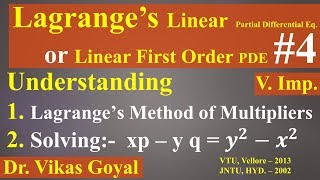
Lagrange's method provides a systematic approach to find the general solution of first-order linear PDEs by integrating auxiliary equations derived from the standard form of the PDE. Key examples illustrate the process and outcomes.
Detailed
Overview of Lagrange's Method in First-Order Linear PDEs
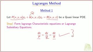
Lagrange's method is a robust technique applied to solve first-order linear partial differential equations (PDEs) of the form:
\[ P(x,y,z) \frac{\partial z}{\partial x} + Q(x,y,z) \frac{\partial z}{\partial y} = R(x,y,z) \]
To find solutions, we utilize auxiliary equations represented as:
\[ \frac{dx}{P} = \frac{dy}{Q} = \frac{dz}{R} \]
These equations are ordinary differential equations (ODEs) that facilitate the derivation of the general solution for the PDE. An example provided illustrates this method in action:
- Given PDE Example: \( \frac{\partial z}{\partial x} + \frac{\partial z}{\partial y} = 0 \)
- Auxiliary Equations: \( \frac{dx}{1} = \frac{dy}{1} = \frac{dz}{0} \)
- Solving these yields the relationships \( x - y = c \) and \( z = c \), leading to the general solution represented by \( z = f(x-y) \).
This method emphasizes the integration of results from auxiliary equations to derive solutions, demonstrating its practical application in mathematical modeling.
Youtube Videos


Audio Book
Dive deep into the subject with an immersive audiobook experience.
Standard Form of First-Order Linear PDE
Chapter 1 of 3
🔒 Unlock Audio Chapter
Sign up and enroll to access the full audio experience
Chapter Content
The standard form is:
∂z ∂z
P(x,y,z) + Q(x,y,z) = R(x,y,z)
∂x ∂y
Detailed Explanation
In studying Partial Differential Equations (PDEs), particularly first-order linear PDEs, we start by expressing the equation in a standard form. This form typically includes a function of several variables, here denoted as P, Q, and R, which represent coefficients of the partial derivatives taken with respect to x and y. This organization helps in systematically analyzing and finding solutions to the equation.
Examples & Analogies
Think of this standard form like a recipe where P, Q, and R are ingredients. Each ingredient contributes differently to the final dish (solution) based on how they interact (the operation of differentiation) with the main components (the variables). Just like a recipe is essential for a successful meal, this standard form is crucial for solving the PDE.
Integrating the Auxiliary Equations
Chapter 2 of 3
🔒 Unlock Audio Chapter
Sign up and enroll to access the full audio experience
Chapter Content
Solution: Integrate the auxiliary equations:
dx dy dz
= =
P Q R
Detailed Explanation
After establishing the standard form of the PDE, we derive auxiliary equations that lead us to find a solution. This involves setting up a system of ordinary differential equations (ODEs) represented as dx/dP = dy/Q = dz/R. By integrating these equations, we can obtain a general solution to the original PDE.
Examples & Analogies
Consider solving this PDE like navigating a treasure map (the auxiliary equations) where each coordinate (dx, dy, dz) guides you to the next step. By carefully following these coordinates and integrating them, you gradually uncover the path to your 'treasure' (the general solution) along the way.
Example of Lagrange’s Method
Chapter 3 of 3
🔒 Unlock Audio Chapter
Sign up and enroll to access the full audio experience
Chapter Content
Example:
Given: ∂z + ∂z = 0
∂x ∂y
→ Lagrange’s auxiliary equations:\ndx dy dz
= =
1 1 0
Solving gives: x−y = c, z = c
Hence, the general solution: z = f(x−y)
Detailed Explanation
To illustrate how Lagrange's method works, we parse a specific example involving the equation ∂z/∂x + ∂z/∂y = 0. From it, we derive the auxiliary equations, indicating the relationships between the differentials dx, dy, and dz. By solving these equations, we find that x - y = c and z = c, establishing a general solution that can be represented as z = f(x - y), where f is an arbitrary function. This indicates a family of solutions based on the constant 'c'.
Examples & Analogies
Think of f(x - y) like a family of trees (solutions) growing according to their location (coordinates) where each tree represents a different situation or condition based on the relationship defined by x - y = c. Just as trees adapt to their surroundings while still sharing a common characteristic (the type of tree), the different functions produced from f illustrate varied yet related solutions to the same underlying PDE.
Key Concepts
-
First-Order Linear PDE: A form of PDE involving first-order derivatives.
-
Lagrange’s Method: A systematic approach to solving first-order linear PDEs.
-
Auxiliary Equations: Equations that simplify the process of integrating to find solutions.
Examples & Applications
Solving the equation \( \frac{\partial z}{\partial x} + \frac{\partial z}{\partial y} = 0 \) using auxiliary equations to derive its general solution.
Finding relationships among variables using integration from auxiliary equations.
Memory Aids
Interactive tools to help you remember key concepts
Rhymes
A PDE first-order is a simple score, Lagrange’s method opens the door!
Stories
Imagine a mathematician named Lagrange who found a shortcut through a complex equation maze, leading to clear paths of solutions!
Acronyms
Remember 'AID' for 'Auxiliary Integrate Derive!'
Flash Cards
Glossary
- FirstOrder Linear PDE
A partial differential equation that involves the first derivatives of an unknown function.
- Lagrange's Method
A technique to solve first-order linear PDEs by transforming them into auxiliary ordinary differential equations.
- Auxiliary Equations
Equations derived from the standard form of a PDE that facilitate the integration process to find solutions.
Reference links
Supplementary resources to enhance your learning experience.