
Worked Example – Wave Equation
Enroll to start learning
You’ve not yet enrolled in this course. Please enroll for free to listen to audio lessons, classroom podcasts and take practice test.
Interactive Audio Lesson
Listen to a student-teacher conversation explaining the topic in a relatable way.
Understanding the Wave Equation
🔒 Unlock Audio Lesson
Sign up and enroll to listen to this audio lesson

Today, we are going to learn about the one-dimensional wave equation, which describes how waves propagate. The equation is represented as ∂²u/∂t² = c²∂²u/∂x². Can anyone tell me what each term represents?

The 'u' typically represents the displacement of the wave, right?

And 'c' is the speed of the wave? How does that affect the wave propagation?
Exactly! 'c' is the wave speed, which dictates how fast the disturbance travels through the medium. Remember, the wave equation is essential in understanding phenomena like sound waves and vibrations in structures!
Boundary Conditions
🔒 Unlock Audio Lesson
Sign up and enroll to listen to this audio lesson

Next, let’s discuss boundary conditions. For this problem, we have u(0, t) = 0 and u(L, t) = 0. What do these conditions imply?

That means the wave is fixed at both ends?

So the endpoints of the string do not move, creating standing waves!
Exactly! This is crucial for understanding how the wave will behave in a physical medium.
Initial Conditions
🔒 Unlock Audio Lesson
Sign up and enroll to listen to this audio lesson
When solving PDEs, we often need initial conditions. Here, we have u(x, 0) = f(x) and ∂u/∂t(x, 0) = g(x). What do these conditions allow us to do?
They give us the initial state of the wave?
And they help determine unique solutions for our constants like A_n and B_n later on!
Exactly! These conditions are essential for tailoring the solution to the specific problem we are exploring.
Separation of Variables
🔒 Unlock Audio Lesson
Sign up and enroll to listen to this audio lesson
Now let’s look at the method of separation of variables. We assume u(x, t) = X(x)T(t). Can anyone explain why we can do this?
Because we want to solve for X and T in two separate equations!
It simplifies the problem into more manageable ordinary differential equations!
Great explanations! By separating the variables, we can solve each part independently and combine the solutions.
Constructing the Final Solution
🔒 Unlock Audio Lesson
Sign up and enroll to listen to this audio lesson
After solving for X(x) and T(t), we combine them to find the complete solution to the wave equation. Does anyone recall the form of the solution we derive?
It looks like a series with sines and cosines! Something like an infinite sum, right?
Yes! And the coefficients A_n and B_n are determined from the initial conditions using Fourier series!
Absolutely correct! This method reveals how the wave behaves over time in a bounded medium, which is crucial in engineering applications.
Introduction & Overview
Read summaries of the section's main ideas at different levels of detail.
Quick Overview
Standard
In this section, the one-dimensional wave equation is examined via a detailed worked example. The solution incorporates boundary conditions and initial conditions, illustrating the method of separation of variables and the resulting form of the solution, emphasizing its applications in modeling vibrations in structures.
Detailed
Worked Example – Wave Equation
Introduction
In this section, we explore the one-dimensional wave equation, a fundamental equation widely used in engineering applications. The wave equation describes how waves, such as sound waves or vibrations in strings, propagate through space. Our goal is to solve the wave equation under given boundary and initial conditions, providing a clear framework for understanding its application in real-world scenarios.
Wave Equation
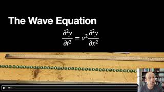
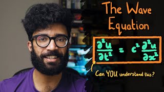
The wave equation in one dimension is given by:
$$\frac{\partial^2 u}{\partial t^2} = c^2 \frac{\partial^2 u}{\partial x^2} , \quad 0 < x < L, \quad t > 0$$
with:
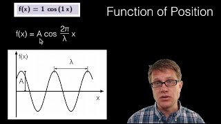
- $u(x, t)$ being the displacement at position $x$ and time $t$.
- $c$ representing the wave speed.
Boundary Conditions
We impose the following boundary conditions:
- $u(0, t) = 0$ (displacement is zero at the left end)
- $u(L, t) = 0$ (displacement is zero at the right end)
These conditions are consistent with a fixed string or beam at both endpoints.
Initial Conditions
To uniquely determine the solution, we define initial conditions:
- $u(x, 0) = f(x)$ (initial shape of the wave)
- $\frac{\partial u(x, 0)}{\partial t} = g(x)$ (initial velocity of the wave)
Solution Method
Assuming a separable solution of the form:
$$u(x, t) = X(x) T(t)$$
we substitute into the wave equation, yielding:
$$\frac{T''(t)}{c^2 T(t)} = \frac{X''(x)}{X(x)} = -\lambda$$
where $\lambda$ is a separation constant. Solving these ordinary differential equations results in:
- X-Equation: $X(x) = sin(\frac{n\pi x}{L})$, $\lambda = (\frac{n\pi}{L})^2$ for $n = 1, 2, 3, ...$
- T-Equation: $T(t) = A_n cos(c \sqrt{\lambda} t) + B_n sin(c \sqrt{\lambda} t)$
Complete Solution
The complete solution of the wave equation can be expressed as:
$$u(x, t) = \sum_{n=1}^{\infty} [A_n cos(\frac{n\pi ct}{L}) + B_n sin(\frac{n\pi ct}{L})] sin(\frac{n\pi x}{L})$$
Final Note
To find specific values for $A_n$, and $B_n$, Fourier series methods are applied based on the initial conditions, leading to a comprehensive understanding of wave propagation in bounded media.
Youtube Videos


Audio Book
Dive deep into the subject with an immersive audiobook experience.
Problem Statement
Chapter 1 of 4
🔒 Unlock Audio Chapter
Sign up and enroll to access the full audio experience
Chapter Content
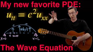
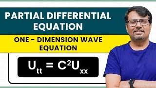
Solve the one-dimensional wave equation:
\[ \frac{\partial^2 u}{\partial t^2} = c^2 \frac{\partial^2 u}{\partial x^2}, \quad 0<x
Subject to boundary conditions:
- \( u(0,t)=0, \; u(L,t)=0 \)
- Initial conditions: \( u(x,0)=f(x), \; \frac{\partial u(x,0)}{\partial t}=g(x) \)
Detailed Explanation
In this chunk, we are given a problem to solve the wave equation, which describes how waves propagate through a medium. The wave equation here is a second-order partial differential equation (PDE) that relates the second time derivative and the second spatial derivative of a function \( u \), which usually represents a physical quantity like displacement. The description specifies the behavior of the wave on a segment of a line from 0 to L over time. The boundary conditions indicate that the displacement at both ends (0 and L) must be zero. The initial conditions tell us how the system starts at time t=0, with \( f(x) \) defining the starting shape of the wave and \( g(x) \) defining the initial velocity of the wave.
Examples & Analogies
Think of a plucked guitar string. When you pluck the string, it vibrates to create sound, which is an example of a wave. The wave travels along the string between two fixed points (the ends of the string). The equation describes how the string vibrates over time and how its shape and velocity evolve as the wave travels.
Assumption of Separation of Variables
Chapter 2 of 4
🔒 Unlock Audio Chapter
Sign up and enroll to access the full audio experience
Chapter Content
Assume: \( u(x,t)=X(x)T(t) \)
Substitute into PDE:
\[ T''(t) X(x) = c^2 X''(x) T(t) \] ⇒ = =−λ
\[ c^2 \frac{T(t)}{T(t)} = -\lambda \frac{X(x)}{X(x)} \]
Detailed Explanation
In this step, we use a method called 'separation of variables,' which assumes that the solution to the wave equation can be expressed as a product of a function in space, \( X(x) \), and a function in time, \( T(t) \). When we substitute this assumption into the wave equation, we can separate the variables, leading to two ordinary differential equations. This is done by rearranging the equation into a form where one side contains only terms involving T, and the other side only terms involving X. The resulting equations can often be solved independently.
Examples & Analogies
Imagine you're organizing a dance performance where different dancers perform various parts simultaneously. If you separate the dance into two groups—one group focuses on specific movements (spatial pattern), while the other group focuses on the timing of the music (temporal pattern)—you can analyze and refine each group's performance separately before combining them for the final show.
Solutions for Spatial and Temporal Functions
Chapter 3 of 4
🔒 Unlock Audio Chapter
Sign up and enroll to access the full audio experience
Chapter Content
Solving gives:
- \( X(x)=sin\left(\frac{n\pi x}{L}\right), \; \lambda=(\frac{n\pi}{L})^2 \)
- \( T(t)=A \cos(c \lambda t)+B \sin(c \lambda t) \)
Detailed Explanation
The solution for the spatial part \( X(x) \) results in sinusoidal functions, indicating that the displacement along the string takes the shape of a sine wave. The constant \( n \) corresponds to different modes of vibration, and the parameter \( \lambda \) relates to the frequency of those vibrations. The temporal part \( T(t) \) consists of a combination of sine and cosine functions, which describe how the amplitude changes over time. The parameters \( A \) and \( B \) will be determined based on the initial conditions provided.
Examples & Analogies
Consider how different musical notes (represented by different values of n) create distinct sounds. The vibration patterns of the guitar produce complex sounds over time. The sine and cosine solutions for those vibrations show how each note continues to resonate and fade, similar to how sound from a guitar string evolves as it is plucked.
Complete Solution using Fourier Series
Chapter 4 of 4
🔒 Unlock Audio Chapter
Sign up and enroll to access the full audio experience
Chapter Content
So the complete solution:
\[ u(x,t) = \sum_{n=1}^{\infty} \left[A_n \cos\left(\frac{n\pi ct}{L}\right) + B_n \sin\left(\frac{n\pi ct}{L}\right)\right] \sin\left(\frac{n\pi x}{L}\right) \]
Use Fourier series to determine \( A_n, B_n \) from initial conditions.
Detailed Explanation
The complete solution is expressed as an infinite series, known as a Fourier series, which represents the sum of all possible waveforms at each point in time and space. The Fourier series allows us to reconstruct the overall wave behavior from the individual modes captured by the sine functions. The coefficients \( A_n \) and \( B_n \) will be determined using the initial conditions of the problem (the shape of the wave and its velocity at t=0). This enables us to tailor the general solution to fit the specific physical scenario being modeled.
Examples & Analogies
Pumpkin pie has layers of flavor—from spices to pumpkin sweetness—much like how the Fourier series combines different 'flavors' (sine and cosine components) to create the complete sound of the wave. Each note contributes to the overall taste, just as each sine wave contributes to the overall wave shape over time.
Key Concepts
-
Wave Equation: Describes the propagation of waves and is fundamental in engineering.
-
Boundary Conditions: Defines the behavior at the edges of the medium, crucial for solutions.
-
Initial Conditions: Set the state of the wave at t=0, allowing for a unique solution.
-
Separation of Variables: A method for simplifying the wave equation into solvable parts.
-
Fourier Series: Method used to find coefficients in the solution involving boundary conditions.
Examples & Applications
When a string fixed at both ends is plucked, the wave created can be modeled using the wave equation with boundary conditions reflecting its fixed endpoints.
The vibrations produced in a drum membrane when struck can also be analyzed using the wave equation under appropriate initial conditions.
Memory Aids
Interactive tools to help you remember key concepts
Rhymes
To solve the wave, just be brave, with boundary sets, your answers you'll save.
Stories
Imagine a guitar string. When plucked, it vibrates, but the ends stay fixed. This is where boundary conditions come into play, shaping how the wave travels.
Memory Tools
Remember 'B.I.S.': Boundary conditions, Initial conditions, Separation of variables - the keys to solving PDEs.
Acronyms
C.I.S.
for Complete Initial Solution – remember to always specify your conditions!
Flash Cards
Glossary
- Wave Equation
A second-order partial differential equation that describes the propagation of waves, such as sound or light.
- Boundary Conditions
Conditions that specify the behavior of a wave at the boundaries of the domain.
- Initial Conditions
Conditions that specify the state of the system at the beginning of the observation.
- Separation of Variables
A method used to solve partial differential equations by assuming that the solution can be factored into products of functions of single variables.
- Fourier Series
A series that expresses a function as the sum of sinusoidal components, which aids in solving PDEs with specific boundary conditions.
Reference links
Supplementary resources to enhance your learning experience.