
Method of Separation of Variables
Enroll to start learning
You’ve not yet enrolled in this course. Please enroll for free to listen to audio lessons, classroom podcasts and take practice test.
Interactive Audio Lesson
Listen to a student-teacher conversation explaining the topic in a relatable way.
Introduction to Separation of Variables
🔒 Unlock Audio Lesson
Sign up and enroll to listen to this audio lesson

Today, we will discuss the method of separation of variables, a powerful technique to solve linear partial differential equations. Who can remind us what a PDE is?

It's an equation that involves partial derivatives with respect to multiple variables!
Exactly! Now, the separation of variables allows us to assume a solution of the form $u(x,t) = X(x)T(t)$. Does anyone know why we would want to write solutions this way?

I think it helps to split the equation into simpler parts we can solve independently!
Correct! This separation simplifies our original PDE into ordinary differential equations, which are much easier to handle. Let's keep this in mind as we explore more.
Applying Separation of Variables to the Heat Equation
🔒 Unlock Audio Lesson
Sign up and enroll to listen to this audio lesson

Now let's focus on the heat equation: $\frac{\partial u}{\partial t} = \alpha \frac{\partial^2 u}{\partial x^2}$. How would you apply our separation of variables here?

We assume $u(x,t) = X(x)T(t)$, then we can substitute this into the equation!
Exactly! After substitution, how do we rearrange the equation?

We set up it to separate the terms involving time and space, creating two equations!
Right! This leads us to two ordinary differential equations. Let’s derive those together!
Solving the Separated ODEs
🔒 Unlock Audio Lesson
Sign up and enroll to listen to this audio lesson
Once we have our separated ODEs: $\frac{dT}{dt} + \alpha \lambda T = 0$ and $\frac{d^2 X}{dx^2} + \lambda X = 0$, how do we solve these?
We can solve the first ODE for $T(t)$ using exponential functions based on the characteristic equation!
Great answer! For $X(x)$, how do we typically solve the second ODE?
We would use trigonometric functions if $\lambda$ is positive, right?
Exactly! By understanding these solutions, we can combine them to compose our general solution for the PDE. Let's summarize the method we’ve discussed today.
Final Application and Importance
🔒 Unlock Audio Lesson
Sign up and enroll to listen to this audio lesson
Now that we've outlined the process, what are some real-world applications where we might utilize the separation of variables?
It’s used in heat distribution problems and fluid flow models!
And in vibrating strings or beams as seen in wave equations.
Excellent points! The method plays a vital role in civil engineering, where accurate modeling leads to better designs and safety. Understanding this technique is crucial for all engineers.
Introduction & Overview
Read summaries of the section's main ideas at different levels of detail.
Quick Overview
Standard
In this section, the method of separation of variables is explained as a powerful strategy for dealing with linear PDEs with boundary or initial conditions. By assuming a solution in a product form, the PDE can be transformed into ordinary differential equations (ODEs) that can be solved independently, facilitating the determination of solutions to complex problems.
Detailed
Method of Separation of Variables
The method of separation of variables is a crucial technique for solving linear partial differential equations (PDEs), especially when accompanied by boundary or initial conditions. The core idea involves assuming that the solution to the PDE can be expressed in the form of the product:
$$ u(x,t) = X(x)T(t) $$
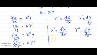
where $X(x)$ is a function dependent on the spatial variable $x$, and $T(t)$ is dependent on time $t$. By substituting this product into the linear PDE, it becomes possible to rearrange the equation to separate the variables. This allows for the division of the equation into two ordinary differential equations (ODEs), one in terms of $X$ and the other in terms of $T$.
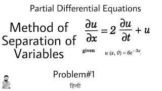
For example, when dealing with the heat equation:
$$ \frac{\partial u}{\partial t} = \alpha \frac{\partial^2 u}{\partial x^2} $$
Assuming the separation of variables with $u(x,t) = X(x)T(t)$ leads to:
$$ \frac{dT}{dt} + \alpha\lambda T = 0 $$
$$ \frac{d^2X}{dx^2} + \lambda X = 0 $$
Here, $\lambda$ represents a separation constant, and each separated equation can be solved independently under specified boundary conditions. The solutions from these ODEs combine to form the general solution to the original PDE, providing insight into the behavior of the physical system modeled by the PDE.
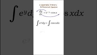
Youtube Videos
Audio Book
Dive deep into the subject with an immersive audiobook experience.
Overview of the Method
Chapter 1 of 5
🔒 Unlock Audio Chapter
Sign up and enroll to access the full audio experience
Chapter Content
A powerful technique used to solve linear PDEs, especially with boundary/initial conditions.
Detailed Explanation
The method of separation of variables is an approach that simplifies solving partial differential equations (PDEs). This technique is particularly useful when the PDE has boundary or initial conditions that need to be satisfied. The essence of the method is to assume that the solution can be broken down into a product of functions, each dependent on a single variable. This allows the PDE to be transformed into simpler ordinary differential equations (ODEs).
Examples & Analogies
Imagine you are trying to bake a cake and you have a recipe that tells you to mix your ingredients correctly based on their types: flour, sugar, and eggs. Just like separating the roles of these ingredients simplifies the baking process, separating variables in a PDE makes it easier to find the solution.
Assumption of Solution Form
Chapter 2 of 5
🔒 Unlock Audio Chapter
Sign up and enroll to access the full audio experience
Chapter Content
Assume a solution of the form: u(x,t)=X(x)T(t)
Detailed Explanation
In the first step of the method, we assume that the function u, which we want to solve for, can be expressed as the product of two functions: X(x) that depends only on the spatial variable x and T(t) that depends only on the time variable t. This assumption helps to transform the multi-variable problem into a simpler form where each variable can be treated independently.
Examples & Analogies
Think of solving a puzzle where you focus on one section at a time instead of trying to complete the whole thing at once. By breaking it down into smaller pieces (X(x) for space and T(t) for time), you make the problem easier to manage and solve.
Substitution into the PDE
Chapter 3 of 5
🔒 Unlock Audio Chapter
Sign up and enroll to access the full audio experience
Chapter Content
Substitute into the PDE, divide both sides to separate variables, and solve resulting ODEs independently.
Detailed Explanation
Once the assumed solution form is substituted into the original PDE, you can manipulate the equation algebraically to isolate the functions X(x) and T(t). Typically, this manipulation leads to a situation where one side of the equation solely consists of the spatial part (X) while the other consists of the temporal part (T). This division indicates that each side can be equal to a constant, leading to separate ordinary differential equations for X and T.
Examples & Analogies
Picture a seesaw where one side represents space and the other side represents time. When you place equal weights on both sides (the constants after separation), it allows you to analyze and balance each side independently, making it easier to understand how each part contributes to the overall system.
Example: Heat Equation
Chapter 4 of 5
🔒 Unlock Audio Chapter
Sign up and enroll to access the full audio experience
Chapter Content
Example:
Heat Equation:
∂u/∂t = α ∂²u/∂x²
Assume u(x,t)=X(x)T(t), substituting gives:
dT/dt + (α/X)d²X/dx² = -λ.
Detailed Explanation
In this example, we look at the heat equation, a common PDE in thermal analysis. By substituting our assumed form u(x,t) = X(x)T(t) into the heat equation and organizing it, we arrive at a form where we can separately analyze the time-dependent behavior (T(t)) and the spatial behavior (X(x)). This separation leads to two ordinary differential equations, which can be solved independently under given boundary conditions.
Examples & Analogies
Imagine you're learning how to play a musical instrument. At first, you practice the melody (the time-dependent aspect) separately from the rhythm (the spatial aspect). By mastering each part individually before combining them, you improve your overall performance, similar to how one solves different parts of the PDE separately for better understanding.
Resulting Ordinary Differential Equations
Chapter 5 of 5
🔒 Unlock Audio Chapter
Sign up and enroll to access the full audio experience
Chapter Content
This leads to two ordinary differential equations:
• dT/dt + αλT = 0
• d²X/dx² + λX = 0
Solve both under given boundary conditions.
Detailed Explanation
The two resulting ordinary differential equations arise from the separation of variables. The first ODE describes how the temperature evolves over time, while the second describes the spatial distribution of temperature. These ODEs can be solved using standard methods from ordinary differential equations, such as finding eigenvalues and eigenfunctions, which ultimately help in determining the full solution to the original PDE under specified boundary conditions.
Examples & Analogies
Think about solving a math problem in two stages: first, you solve for time using simple algebra, and then you tackle the geometry of the problem by breaking it down into shapes. This segmented approach allows you to handle each type of calculation more effectively, leading to a complete solution.
Key Concepts
-
Separation of Variables: A method for solving PDEs by splitting variables.
-
Application to PDEs: Specifically useful for heat and wave equations with initial and boundary conditions.
-
Boundary and Initial Conditions: Essential for determining unique solutions using separation of variables.
Examples & Applications
Assuming $u(x,t) = X(x)T(t)$ in the heat equation leads to two ODEs that can be solved independently under the conditions given.
$X(x) = A ext{sin} (n rac{ ext{π}}{L}x)$ and $T(t) = B ext{e}^{- ext{α}(-n^2 rac{ ext{π}}{L})t}$ represent solutions derived from separating the heat equation.
Memory Aids
Interactive tools to help you remember key concepts
Rhymes
When variables separate their ways, the solution brightens the cloudy days.
Stories
Imagine a puzzle box where you need to divide the pieces based on color and shape before putting it together. This is how we separate our variables!
Memory Tools
S.E.P.A.R.A.T.E: Solve Each Part As Respective And Time-dependent Equations.
Acronyms
U.S. (U = X.T)
Understand Separation keeps it simple!
Flash Cards
Glossary
- Partial Differential Equation (PDE)
An equation that involves partial derivatives of a function with respect to multiple independent variables.
- Ordinary Differential Equation (ODE)
An equation involving derivatives of a function with respect to one variable.
- Separation of Variables
A technique used to solve PDEs by assuming the solution can be expressed as a product of functions, each dependent on a single variable.
- Boundary Condition
Conditions that must be satisfied by the solution of a differential equation at the boundaries of the domain.
- Initial Condition
Condition stating the value of the variables at the initial point, often used in time-dependent problems.
- Eigenvalue
A special scalar value in the context of differential equations that indicates the separation constant.
Reference links
Supplementary resources to enhance your learning experience.