
Gram-Schmidt Orthogonalization
Enroll to start learning
You’ve not yet enrolled in this course. Please enroll for free to listen to audio lessons, classroom podcasts and take practice test.
Interactive Audio Lesson
Listen to a student-teacher conversation explaining the topic in a relatable way.
Introduction to Gram-Schmidt
🔒 Unlock Audio Lesson
Sign up and enroll to listen to this audio lesson

Today we will discuss the Gram-Schmidt orthogonalization process. Can anyone tell me the importance of transforming a set of vectors into an orthonormal set?

It helps in simplifying calculations, especially in linear algebra and engineering work!
Correct! An orthonormal basis simplifies calculations. Now, who can define orthonormal vectors?

Orthonormal vectors are those vectors that are both orthogonal and of unit length.
Exactly! Let's discuss how we can transform a set of linearly independent vectors using this process.
Process Steps
🔒 Unlock Audio Lesson
Sign up and enroll to listen to this audio lesson

We'll begin with our set of linearly independent vectors. The first step is simply to take the first vector and normalize it. Do you remember how to calculate its magnitude?

Yes! You would use the square root of the sum of the squares of its components.
Right! After normalizing the first vector to get \(u_1\), how do we proceed for the next vector?

We need to project the vector onto the previously computed orthonormal vectors?
Exactly! That's the key here. Each new vector is adjusted by subtracting the projections onto all previous orthonormal vectors.
Understanding Projections
🔒 Unlock Audio Lesson
Sign up and enroll to listen to this audio lesson
Now let's discuss vector projections. How do we calculate the projection of a vector \(v_k\) onto an orthonormal vector \(u_i\)?
It’s the scalar product of the two vectors divided by the magnitude of the vector being projected onto, times that vector.
Correct! It's given by \(\text{proj}_{u_i}(v_k) = \frac{v_k \cdot u_i}{u_i \cdot u_i} u_i\). Can someone tell me why we normalize \(u_k\) after adjusting?
To ensure that our vectors remain unit vectors after the adjustments.
Great! Normalization is essential to maintain the orthonormal property of the basis.
Final Thoughts on Orthonormal Basis
🔒 Unlock Audio Lesson
Sign up and enroll to listen to this audio lesson
To wrap up, what do you think is the final outcome of applying the Gram-Schmidt process on a set of vectors?
We end up with an orthonormal basis that we can use for easier computations!
That's right! This orthonormal basis facilitates numerous applications in mathematics and engineering. How confident do you feel now about the Gram-Schmidt process?
I feel much more confident now, especially understanding the significance behind each step.
Fantastic! Remember, it's a powerful tool in the context of vector spaces.
Introduction & Overview
Read summaries of the section's main ideas at different levels of detail.
Quick Overview
Standard
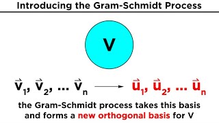
The Gram-Schmidt orthogonalization process gradually constructs an orthonormal set of vectors from an initial set of linearly independent vectors, ensuring that each new vector is orthogonal to the previous ones through vector projections.
Detailed
Gram-Schmidt Orthogonalization
The Gram-Schmidt orthogonalization process is a method that takes a finite set of linearly independent vectors and transforms them into an orthonormal set. This is particularly useful in various areas of mathematics and engineering as it simplifies the representation of data and facilitates calculations.
Steps of the Gram-Schmidt Process:
- Start with a Set of Vectors: Consider a set of linearly independent vectors \(\{v_1, v_2, \ldots, v_n\}\).
- Construct the First Orthonormal Vector: The first orthonormal vector \(u_1\) is simply the first vector normalized:
\[ u_1 = \frac{v_1}{\|v_1\|} \] - Construct Subsequent Vectors: Each subsequent vector is computed as follows:
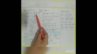
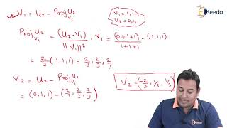
\[ u_k = \frac{v_k - \text{proj}{u_1}(v_k) - \text{proj}{u_2}(v_k) - \ldots - \text{proj}{u{k-1}}(v_k)}{\|v_k - \text{proj}{u_1}(v_k) - \text{proj}{u_2}(v_k) - \ldots - \text{proj}{u{k-1}}(v_k)\|} \]
where \( \text{proj}_{u_i}(v_k) = \frac{v_k \cdot u_i}{u_i \cdot u_i} u_i \) denotes the projection of \(v_k\) onto the previously computed orthonormal vectors. - Repeat: Continue this process until all vectors have been processed, resulting in an orthonormal basis \(\{u_1, u_2, \ldots, u_n\}\).
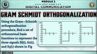
This method is significant for simplifying data representations and is widely employed in numerical methods, including QR factorization and various applications in engineering.
Youtube Videos
Audio Book
Dive deep into the subject with an immersive audiobook experience.
Introduction to Gram-Schmidt Orthogonalization
Chapter 1 of 3
🔒 Unlock Audio Chapter
Sign up and enroll to access the full audio experience
Chapter Content
Given a set of linearly independent vectors {v_1, v_2, ..., v_n}, this process constructs an orthonormal basis {u_1, u_2, ..., u_n} such that:
Detailed Explanation
The Gram-Schmidt process is a method used to convert a set of linearly independent vectors into an orthonormal set. This means that not only are the vectors independent, but they are also orthogonal (perpendicular) to each other and each vector has a length of one. The process starts with a group of vectors in a vector space and modifies them step by step to form the new orthonormal basis.
Examples & Analogies
Imagine you have several pieces of a puzzle. Each piece represents a vector. While they might fit together (independent), they may not all be shaped the same way (orthogonal). Using the Gram-Schmidt process is like reshaping the pieces so they not only fit together perfectly but also fill the space neatly without overlapping, allowing all paths to connect without interference.
Construction of Orthonormal Basis
Chapter 2 of 3
🔒 Unlock Audio Chapter
Sign up and enroll to access the full audio experience
Chapter Content
v_1 = u_1, u_1 = \frac{v_1}{\|v_1\|},
v_2 = v_2 - \text{proj}{u_1}(v_2), u_2 = \frac{v_2}{\|v_2 - \text{proj}{u_1}(v_2)\|},...
Detailed Explanation
To form the orthonormal basis from the original vectors, we first take the first vector, v_1, and normalize it to get u_1. This involves dividing v_1 by its length (magnitude) to ensure u_1 has a length of 1. The next step modifies v_2 by subtracting its projection on u_1, making it orthogonal to u_1. Then, we normalize this new vector to create u_2. This process can be repeated for all subsequent vectors, ensuring that each resulting vector is orthogonal to all previous vectors and of unit length.
Examples & Analogies
Think of the first vector as a direction in a forest. You establish a clear trail (u_1) by marking your first path. When you add a second path (v_2), you need to ensure it doesn't overlap or cross paths with the first. You clear the underbrush (subtract projections) that might lead to confusion and keep the second path neat and clear (normalized as u_2). Each new path you create must respect the previous ones, maintaining a beautiful layout of distinct trails that showcase the forest's depth.
Projection and Normalization
Chapter 3 of 3
🔒 Unlock Audio Chapter
Sign up and enroll to access the full audio experience
Chapter Content
where: v \cdot u \text{ and } \text{proj}(v) = \frac{v \cdot u}{u \cdot u} u.
Detailed Explanation
In the process, we utilize projections to modify the vectors. The projection of one vector onto another helps us understand how much of one vector goes in the direction of another. This is important when we want to remove components of vectors that are aligned in the same direction. The formula for projection uses the dot product to calculate this overlapping part, resulting in a clear imagery of the relationship between the two vectors involved.
Examples & Analogies
Imagine trying to cast a shadow of a tree onto a wall. The shadow represents the projection you create by angling a light source. By understanding and manipulating this shadow, you can adjust how it interacts with other elements in the scene, ensuring each form stands out. In the same way, projections help us clarify how vectors extend into their space, allowing for more precise representation in our new orthonormal basis.
Key Concepts
-
Gram-Schmidt Process: A sequence of steps that transforms a set of linearly independent vectors into an orthonormal basis.
-
Projection: The way to find the component of one vector in the direction of another.
-
Orthonormal Basis: A basis consisting of orthogonal vectors, each of length one.
Examples & Applications
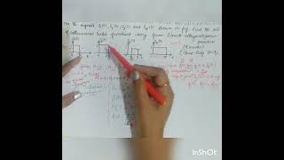
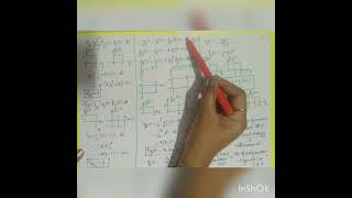
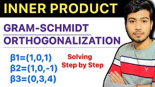
Example of transforming a set of vectors \{(1, 0), (1, 1)\} into an orthonormal set using Gram-Schmidt.
Given vectors \{(1, 1, 0), (0, 1, 1)\}, the Gram-Schmidt process generates orthonormal vectors.
Memory Aids
Interactive tools to help you remember key concepts
Rhymes
Gram-Schmidt, we align, vectors stand, so fine, when they norm and project, orthonormal we connect.
Stories
Imagine a team of vectors struggling to fit together. With the Gram-Schmidt coach, they learn to respect each other’s space, aligning themselves to create a harmonious, orthonormal team.
Memory Tools
Use the acronym 'NPA' - Normalize, Project, Adjust when recalling steps in the Gram-Schmidt process.
Acronyms
GSO - Gram-Schmidt Orthogonalization for remembering key steps in the orthogonalization process.
Flash Cards
Glossary
- Orthonormal Vectors
Vectors that are both orthogonal (perpendicular) and have unit length.
- Linearly Independent Vectors
A set of vectors where no vector can be expressed as a linear combination of others.
- Projection
The process of mapping a vector onto another vector.
- Basis
A set of vectors that linearly independent spans a vector space.
Reference links
Supplementary resources to enhance your learning experience.