
CONTINUOUS CHARGE DISTRIBUTION
Enroll to start learning
You’ve not yet enrolled in this course. Please enroll for free to listen to audio lessons, classroom podcasts and take practice test.
Interactive Audio Lesson
Listen to a student-teacher conversation explaining the topic in a relatable way.
Calculating Electric Fields from Continuous Charge Distributions
🔒 Unlock Audio Lesson
Sign up and enroll to listen to this audio lesson

To find the electric field from continuous charge distributions, we can use Coulomb’s law combined with integration. Can anyone remind me how Coulomb's law applies here?

Isn't it about calculating the force between charges?
Yes! But in this case, we are looking for the field created by a distribution of charge. We take small volume elements and apply the law to each.

So we would use dE, right?
"Correct! We can calculate the electric field contribution from each volume element as:
Introduction & Overview
Read summaries of the section's main ideas at different levels of detail.
Quick Overview
Standard
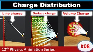
The section explores the limitations of using discrete charge configurations and introduces continuous charge distributions as a more practical approach. It defines surface, line, and volume charge densities and describes how to calculate electric fields using Coulomb's law and the superposition principle.
Detailed
Continuous Charge Distribution
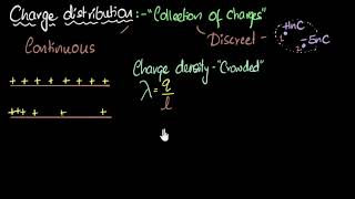
In this section, we shift our focus from discrete charge configurations, which involve isolated charges like q1, q2, ..., qn, to continuous charge distributions that are essential for practical applications, especially on macroscopic scales. Instead of analyzing individual charges, we consider areas, lines, or volumes of space where charge is distributed continuously.
Key Definitions:
- Surface Charge Density (σ): This is defined for charged surfaces where we consider an infinitesimally small area element, DS, and represent it with the following formula:
σ = ΔQ / ΔS
where ΔQ is the charge on the area element ΔS, with units C/m².
- Linear Charge Density (λ): For a wire or line charge, we consider small line elements, Δl, and define the linear charge density as:
λ = ΔQ / Δl
where the units are C/m.
- Volume Charge Density (ρ): For bulk materials, we represent charge distribution in a three-dimensional volume, defined similarly by:
ρ = ΔQ / ΔV
with units C/m³.
Calculating Electric Fields:
To find the electric field due to a continuous charge distribution, we proceed similarly to the discrete charge case using Coulomb's law. By dividing the charge distribution into small volume elements, we can apply the superposition principle to sum the contributions to the electric field at a point P from various volume elements.
- Use:
dE = (1/(4πε₀)) * (ρ dv) / r²
where ρ is the charge density, dv is the volume element, and r is the distance to the point P.
- A final integral will give us the total electric field due to the entire distribution:
E = ∫(dE)
In conclusion, while continuous charge distributions are conceptually more complex than discrete charges, they provide a useful framework for analyzing electric fields and charge interactions at larger scales.
Youtube Videos


Audio Book
Dive deep into the subject with an immersive audiobook experience.
Defining Continuous Charge Distribution
Chapter 1 of 4
🔒 Unlock Audio Chapter
Sign up and enroll to access the full audio experience
Chapter Content
We have so far dealt with charge configurations involving discrete charges q₁, q₂, ..., qₙ. One reason why we restricted to discrete charges is that the mathematical treatment is simpler and does not involve calculus. For many purposes, however, it is impractical to work in terms of discrete charges and we need to work with continuous charge distributions.
Detailed Explanation
In this chunk, we establish the need to transition from discrete charged particles to a more practical consideration of continuous charge distributions. Continuous charge distributions simplify the analysis of systems where charge is spread over a surface or volume, which is often the case in real-world applications such as charged conductors or electric fields around shapes.
Examples & Analogies
Think of a water pipe with water flowing through it. We often measure the overall flow rate rather than counting each individual water molecule. Similarly, for charged objects, especially those where charge is distributed, it’s more efficient to consider the overall distribution than to consider each individual charge.
Surface Charge Density
Chapter 2 of 4
🔒 Unlock Audio Chapter
Sign up and enroll to access the full audio experience
Chapter Content
For example, on the surface of a charged conductor, it is impractical to specify the charge distribution in terms of the locations of the microscopic charged constituents. It is more feasible to consider an area element DS on the surface of the conductor (which is very small on the macroscopic scale but big enough to include a very large number of electrons) and specify the charge DQ on that element. We then define a surface charge density σ at the area element by σ = DQ/DS.
Detailed Explanation
Here, we introduce the concept of surface charge density, which is a measure of how much charge is distributed over a particular area of the surface. This concept is especially useful in electromagnetic applications, where understanding the distribution of charge on surfaces is crucial for determining electric fields and forces around those surfaces.
Examples & Analogies
Imagine you have a large sponge soaked with water. The amount of water on the sponge surface at any point is like the surface charge density; you can think of how much liquid covers a small area of the sponge compared to the entire sponge. This allows us to simplify the problem to just looking at portions of the sponge rather than the entire volume.
Volume Charge Density
Chapter 3 of 4
🔒 Unlock Audio Chapter
Sign up and enroll to access the full audio experience
Chapter Content
Similar considerations apply for a line charge distribution and a volume charge distribution. The volume charge density (sometimes simply called charge density) is defined in a similar manner: ρ = DQ/DV where DQ is the charge included in the macroscopically small volume element DV that includes a large number of microscopic charged constituents. The units for ρ are C/m³.
Detailed Explanation
Volume charge density refers to the amount of charge per unit volume, allowing us to analyze the effects of charge spread throughout a three-dimensional space rather than on a surface alone. By averaging the distribution over small but significant volumes, we can simplify analysis tasks in complex charge distributions.
Examples & Analogies
Think of a fruit juice blend. Instead of examining each droplet of juice, you consider the concentration of juice per liter. This average gives you a more manageable way to understand how strong the flavor is throughout the drink, similar to how charge density helps simplify electrical calculations.
Calculating Electric Field from Continuous Charge Distribution
Chapter 4 of 4
🔒 Unlock Audio Chapter
Sign up and enroll to access the full audio experience
Chapter Content
The field due to a continuous charge distribution can be obtained in much the same way as for a system of discrete charges. Suppose a continuous charge distribution in space has a charge density ρ. Choose any convenient origin O and let the position vector of any point in the charge distribution be r. Divide the charge distribution into small volume elements of size DV. The charge in a volume element DV is ρDV. Now, consider any general point P (inside or outside the distribution) with position vector R. Electric field due to the charge ρDV is given by Coulomb’s law: DE = (1/4πε₀) * (ρDV)/r'², where r' is the distance between the charge element and P, and ρ' is a unit vector in the direction from the charge element to P.
Detailed Explanation
This chunk discusses the mathematical approach to find the electric field created by a continuous charge distribution. By dividing the distribution into infinitesimally small elements, we can apply Coulomb’s law to each of these elements and then sum up their contributions. This process leads to an integral that provides the total electric field at a point resulting from the entire distribution.
Examples & Analogies
Imagine trying to determine how far sound travels in a crowded stadium. You wouldn't listen to each person’s voice individually; rather, you'd consider the collective crowd noise in sections. Similarly, the electric field calculations involve summing up contributions from all parts of a charge distribution to get an aggregate effect.
Key Concepts
-
Continuous Charge Distribution: Describes how charge can be distributed over areas, lines, or volumes rather than just as discrete charges.
-
Surface Charge Density (σ): Charge per unit area used to define charge distribution on surfaces.
-
Linear Charge Density (λ): Charge per unit length for line distributions, especially in wires.
-
Volume Charge Density (ρ): Charge per unit volume, useful for bulk materials.
-
Electric Field Calculation: The method of finding electric fields through integration of contributions from continuous charge distributions using Coulomb's law.
Examples & Applications
Calculating the electric field from a uniformly charged thin wire by integrating contributions from small segments of charge along its length.
Determining the surface charge density on a charged conductor by measuring the total charge and the area.
Memory Aids
Interactive tools to help you remember key concepts
Rhymes
For surface charge dense, on an area we commence; for linear, length we sense, and volume fills the immense.
Stories
Imagine a park where kids distribute candies. Some on the ground, some in a line to a stand, and some filling a large container. Each represents surface, line, and volume charge densities!
Memory Tools
Silly Little Vanimals: S (Surface), L (Linear), V (Volume) help to remember the charge densities.
Acronyms
Daisy
(Density)
(Charge)
(Area)
(Length)
and V (Volume) to remember how charge is measured and distributed.
Flash Cards
Glossary
- Surface Charge Density (σ)
Charge distributed over a surface area, defined as σ = ΔQ / ΔS (C/m²).
- Linear Charge Density (λ)
Charge distributed along a line, given by λ = ΔQ / Δl (C/m).
- Volume Charge Density (ρ)
Charge distributed in a volume, defined as ρ = ΔQ / ΔV (C/m³).
- Electric Field (E)
A vector field around charged particles that exerts force on other charges.
- Coulomb's Law
The law that describes the force between two charges, foundational for calculating electric fields.
Reference links
Supplementary resources to enhance your learning experience.