
Computational Complexity of the Radix-2 FFT
Interactive Audio Lesson
Listen to a student-teacher conversation explaining the topic in a relatable way.
Introduction to Computational Complexity
🔒 Unlock Audio Lesson
Sign up and enroll to listen to this audio lesson

Today, we're going to explore the computational complexity of the Radix-2 FFT. Can anyone recall what we mean by 'computational complexity'?

Is it how much time or resources an algorithm needs to complete its task?
Exactly! It's about understanding the resources required as the size of the input data grows. With the Radix-2 FFT, we look at operations needed to compute the DFT.

How does it compare to the direct DFT computation?
Great question! The direct computation of the DFT takes O(N²). The Radix-2 FFT reduces that dramatically to O(N log N).

Wow, that sounds like a huge difference!
It is! This efficiency is crucial for large datasets where computations can otherwise be prohibitive. Let’s summarize: Radix-2 FFT is significantly more efficient than direct DFT computation.
Recursive Division in Radix-2 FFT
🔒 Unlock Audio Lesson
Sign up and enroll to listen to this audio lesson

Now, let's dive into how the Radix-2 FFT achieves this efficiency. It employs a divide-and-conquer approach. Who can explain what that means?

It means breaking the problem down into smaller parts that are easier to solve.
Correct! In the case of the Radix-2 FFT, it divides the input sequence into even and odd indexed terms.
And then it recursively processes those smaller sequences, right?
Exactly! As we recurse down, we eventually compute a simple two-point DFT. This recursive breakdown is why we get those O(N log N) operations.
Can we visualize how this works in practice?
Sure! Remember, the 'O' notation is just a way to express how the complexity scales as N increases, highlighting efficiency.
Analyzing Complexity Levels
🔒 Unlock Audio Lesson
Sign up and enroll to listen to this audio lesson
Let’s break down the levels of recursion more. How many levels do you think we have with N data points?
Is it log₂(N)?
Correct! Each time we split the DFT, we double the data size, leading to logarithmic levels. Can anyone explain how many operations we perform at each level?
We perform N operations at each level.
Exactly! This is why we combine these two factors to achieve O(N log N) for the entire algorithm.
So, in simple terms, as N gets larger, the number of levels increases but the operations needed at each level do not grow quadratically?
Exactly right! Remembering this hierarchical nature of the FFT is key.
Importance of Efficiency
🔒 Unlock Audio Lesson
Sign up and enroll to listen to this audio lesson
Finally, let’s talk about why all this matters. Why do we care about efficiency in algorithms like FFT?
Because it allows faster computations for larger datasets, which are common in real-world applications!
Exactly! In fields like signal processing, even a small increase in efficiency can lead to significant performance improvements.
So, are we saying that FFT could help in things like audio processing or image analysis?
Yes! That’s the practical significance of learning about these computational complexities. Every millisecond saved can enhance real-time applications.
I see now how essential understanding the concepts behind FFT is!
Absolutely! To sum up, the effectiveness of the Radix-2 FFT transforms the way we handle vast amounts of data quickly and accurately.
Introduction & Overview
Read summaries of the section's main ideas at different levels of detail.
Quick Overview
Standard
This section explains how the Radix-2 FFT efficiently reduces the computational complexity of DFT calculations. By employing a divide-and-conquer strategy that splits the input into even and odd indexed parts, the FFT achieves a much lower operation count, enhancing performance for large datasets.
Detailed
Computational Complexity of the Radix-2 FFT
The computational complexity of the Radix-2 FFT is a significant improvement over the direct computation of the DFT. Let's analyze how the number of operations changes with increasing size of the input, denoted as N:
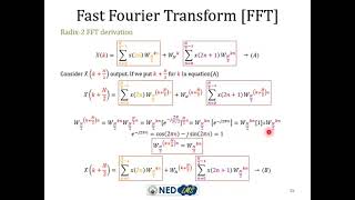
- Recursive Division: At each level of recursion, the Radix-2 FFT divides the computation into two smaller DFTs.
- Number of Levels: The total number of levels in the recursion is logarithmic in relation to N, specifically log₂(N).
- Operations Per Level: Each level involves a linear number of operations, equating to N.
Given these aspects, the total computational effort required by the Radix-2 FFT is expressed as:
O(N log₂(N)).
This is a tremendous reduction from the O(N²) complexity that characterizes direct DFT computation, showcasing the FFT’s efficiency and its suitability for analyzing large datasets.
Youtube Videos
![Decimation In Time - Fast Fourier Transform [Lec 2]](https://img.youtube.com/vi/XeJXx-Te1Eo/mqdefault.jpg)
Audio Book
Dive deep into the subject with an immersive audiobook experience.
Overview of Computational Complexity
Chapter 1 of 5
🔒 Unlock Audio Chapter
Sign up and enroll to access the full audio experience
Chapter Content
The computational complexity of the Radix-2 FFT is significantly reduced compared to the direct computation of the DFT. Let’s consider how the number of operations scales with NN:
Detailed Explanation
In this section, we start by understanding what 'computational complexity' means in the context of algorithms. It refers to how the amount of computing resources required (like time or operations) increases as the size of the input grows. For the Radix-2 FFT algorithm, this complexity is notably lower than that of the direct computation of the Discrete Fourier Transform (DFT). Specifically, it explains that we will analyze how the required number of operations relates to the size of the input, represented as 'N'.
Examples & Analogies
Imagine you're tasked with counting the number of books in a library. If the library has 1000 books, it would take much longer to count them one by one than if the library had only 10 books. This is similar to how computational complexity works — as the number of books (or input size) increases, the time and effort required also increase, but some counting methods (like grouping books) can make the task faster, just like the Radix-2 FFT does for signal processing.
Recursive Divisions
Chapter 2 of 5
🔒 Unlock Audio Chapter
Sign up and enroll to access the full audio experience
Chapter Content
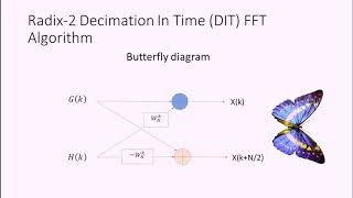
- At each recursive level, the computation is divided into two smaller DFTs.
Detailed Explanation
Here, we delve into how the Radix-2 FFT operates recursively. The core idea is to divide the Fourier Transform calculations into smaller ones. Each time we compute a DFT, we break it down into two smaller DFTs, effectively making it easier to handle. This division continues until we reach the simplest form of the DFT, which has only two data points. By breaking the problem down, we efficiently manage the complexity of the computations.
Examples & Analogies
Think of a large jigsaw puzzle where the pieces are mixed up. Instead of trying to solve the entire puzzle at once, it’s easier to focus on smaller sections first, like the corners or edges, which can be tackled separately. This is similar to how the Radix-2 FFT breaks down the DFT into simpler, manageable parts, making the entire process quicker.
Number of Levels and Operations
Chapter 3 of 5
🔒 Unlock Audio Chapter
Sign up and enroll to access the full audio experience
Chapter Content
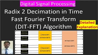
- The number of levels in the recursion is log 2N.
Detailed Explanation
This points out that the recursive division creates a tree-like structure with levels, where the depth of the tree is determined by the logarithm base 2 of N. This logarithmic scaling means that even for large N, the number of levels remains manageable. Each level still requires performing operations, but because of the division, the number of operations is significantly less than in direct computation methods. Therefore, the scaling of operations grows at a much slower rate compared to the size of N.
Examples & Analogies
Imagine you are organizing a tournament where each match eliminates one player. If you start with 16 players, in the first round, you’d have 8 matches, then 4 in the next, and so forth until there’s one winner. Just like with the Radix-2 FFT, where with each round of matches (or calculations) you’re halving the number of players (or data points), leading to a logarithmic number of rounds needed to determine a winner.
Total Operations
Chapter 4 of 5
🔒 Unlock Audio Chapter
Sign up and enroll to access the full audio experience
Chapter Content
- At each level, we perform NN operations.
Detailed Explanation
This statement summarizes the operational workload at each recursive level. It emphasizes that although we are breaking down the problem into smaller parts, each level still requires N operations per small DFT. By considering both the number of operations at each level and the number of levels, we can express the total computation complexity as a function of N, leading us to the conclusion of O(N log_2 N). This expression captures the efficiency increase when using Radix-2 FFT compared to the O(N^2) direct computation.
Examples & Analogies
Continuing with the tournament analogy, while you have fewer players in each round, each match still requires a specific number of efforts (like time, rules interpretations, etc.). Even though the complexity of the entire tournament looks simpler due to fewer matches, you can still estimate the total effort needed by recognizing that every match requires energy (operations) on a consistent scale.
Efficiency Comparison
Chapter 5 of 5
🔒 Unlock Audio Chapter
Sign up and enroll to access the full audio experience
Chapter Content
Thus, the total number of operations is proportional to: O(N log 2N).
Detailed Explanation
Finally, we conclude here by stating the final result of our complexity analysis. The Radix-2 FFT's total operation scales as O(N log_2 N), which is a significant improvement over the O(N^2) complexity of the direct DFT computation. This efficiency means that the Radix-2 FFT can handle larger datasets far more effectively and is vital in real-time applications that rely on quick Fourier transformations.
Examples & Analogies
Consider a factory that produces gadgets. If the factory can make gadgets with a simple machine in 100 hours by going through many steps (O(N^2)), that’s efficient at a smaller scale. But if a new, smarter machine can make them in only 20 hours due to having a faster process (O(N log_2 N)), this makes the factory much better equipped to manage large orders efficiently.
Key Concepts
-
Radix-2 FFT: An efficient algorithm for computing the DFT, reducing complexity to O(N log N).
-
Recursive Division: Splitting the computation into smaller DFTs through a divide-and-conquer approach.
-
Logarithmic Levels: The recursion levels scale as log₂(N), illustrating the computational efficiency.
-
Importance of Efficiency: The Radix-2 FFT enables fast computations essential for real-time data processing.
Examples & Applications
Given a signal of length 8, the Radix-2 FFT will split it into two sequences of length 4, continuing until reaching two-point DFTs.
In audio processing, Radix-2 FFT is used to quickly analyze and manipulate frequency components of sound signals.
Memory Aids
Interactive tools to help you remember key concepts
Rhymes
To break it down and make it fast, Radix-2 will do the task, log N levels, N at each, helps you learn and helps you teach!
Stories
Imagine a village split into halves over a series of nights. Each time they meet, they discover new insights faster and faster — this is how FFT works, halving the problem until it's small enough to solve immediately.
Memory Tools
Remember: F-Or-Complexity-Takes = FFT! (For = Faster and complexity = complexities like O(N log N))
Acronyms
FFT
Fast Function Transformation
Highlighting its speedy nature in transforming functions into frequency space.
Flash Cards
Glossary
- Computational Complexity
A measure of the amount of computational resources required for an algorithm as a function of the size of the input.
- Radix2 FFT
A specific Fast Fourier Transform algorithm that reduces the complexity of the DFT computation by recursively splitting it into smaller parts.
- Discrete Fourier Transform (DFT)
An algorithm used to compute the frequency components of a discrete signal from its time-domain representation.
- O(N log N)
Big O notation representing an upper bound on the time complexity of an algorithm, indicating it scales linearly with N and logarithmically with N.
- O(N²)
Big O notation indicating that an algorithm's runtime is proportional to the square of the input size.
Reference links
Supplementary resources to enhance your learning experience.