
The Radix-2 Cooley-Tukey FFT Algorithm
Interactive Audio Lesson
Listen to a student-teacher conversation explaining the topic in a relatable way.
Breaking the DFT into Even and Odd Parts
🔒 Unlock Audio Lesson
Sign up and enroll to listen to this audio lesson

Today, we're starting with a key concept in the Cooley-Tukey algorithm: breaking the DFT into even and odd parts. Can anyone explain what the DFT is?

DFT stands for Discrete Fourier Transform, right? It converts a sequence of values into frequencies.
Exactly! Now, we can optimize this by separating even and odd indexed terms. When we do this, how do you think it reduces complexity?

I think it allows us to process smaller parts of the DFT at once!
Yes! We end up with two smaller DFTs, which we can compute recursively. Remember the acronym 'EE' for Even and Odd. It’s a neat way to recall their roles in our splits.

So, we rewrite the DFT as combinations of these parts?
Correct! And by defining those new DFTs as X_even and X_odd, we’ve set the stage for our next steps.
To summarize, splitting the DFT allows us to manage calculations better, reducing O(N²) complexity significantly. Let's move on to recursion next!
Recursive Computation of DFTs
🔒 Unlock Audio Lesson
Sign up and enroll to listen to this audio lesson

Now let’s talk about how recursion plays a crucial role in our Radix-2 FFT. What do you think the base case is in this algorithm?
Is it when we reach two-point DFTs?
Exactly! At that point, the DFT calculation is very straightforward. In fact, it's just simple additions and subtractions. Can someone give me the equations involved?

X[0] = x[0] + x[1] and X[1] = x[0] - x[1].
Well done! And remember, this simplicity is key to the speed of the FFT. By repeatedly applying this recursion, we keep dividing until we simplify computations.
So this recursive method is what makes it efficient compared to the direct method?
Absolutely! To recap, recursion allows us to break down the problem into manageable pieces, leading to a significant reduction in computational overhead.
Combining Results
🔒 Unlock Audio Lesson
Sign up and enroll to listen to this audio lesson
Finally, we need to look at how we combine the results of the smaller DFTs. Who remembers the equations we use for combining?
X[k] = X_even[k] + e^(-j2πk/N) * X_odd[k] and X[k + N/2] = X_even[k] - e^(-j2πk/N) * X_odd[k].
Exactly! This relationship is crucial because it enables us to build back up to the full DFT from those smaller parts. Does anyone see why this is effective?
I think it keeps the calculations efficient by reusing the already computed smaller DFTs.
Right again! Reusing smaller computations minimizes repetition, which is the essence of this algorithm's power. Today, we’ve learned how each step builds into the next. What have we covered overall?
We broke the DFT into smaller DFTs, computed them recursively, and combined them to get our final result!
Well summarized! Understanding these steps ensures you can appreciate the Radix-2 FFT's efficiency.
Introduction & Overview
Read summaries of the section's main ideas at different levels of detail.
Quick Overview
Standard
The Radix-2 Cooley-Tukey FFT algorithm reduces the computational complexity of the DFT from O(N²) to O(N log N) through a divide-and-conquer approach. This section elaborates on its derivation by splitting the DFT into even and odd indexed terms, recursive computation, and combining the results.
Detailed
Detailed Summary
The Cooley-Tukey Radix-2 FFT algorithm is a pivotal computational technique in digital signal processing, aimed at efficiently calculating the Discrete Fourier Transform (DFT). The core principle is to decompose the DFT into two smaller DFTs based on the symmetrical properties of complex exponentials. Initially, the sequence is divided into even- and odd-indexed terms, allowing for a simplified and more manageable computation.
Key Steps in the Derivation:
- Breaking the DFT: The DFT sum can be split into two parts: one for even-indexed terms and one for odd-indexed terms. This results in two smaller DFTs, reducing the computational effort significantly.
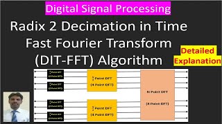
- Recursive Computation: The splitting continues recursively until the base case is reached, where only two-point DFTs are calculated, thus reducing complexity.
- Combining Results: After all smaller DFTs are computed, they are recombined using the recursive relations established, completing the transformation of the original sequence into the frequency domain.
Significance
This algorithm not only accelerates the computation but also expands the avenue for real-time signal processing applications, leading to advancements in areas such as audio analysis, image processing, and telecommunications.
Youtube Videos
![Decimation In Time - Fast Fourier Transform [Lec 2]](https://img.youtube.com/vi/XeJXx-Te1Eo/mqdefault.jpg)
Audio Book
Dive deep into the subject with an immersive audiobook experience.
Step 1: Breaking the DFT into Even and Odd Parts
Chapter 1 of 3
🔒 Unlock Audio Chapter
Sign up and enroll to access the full audio experience
Chapter Content
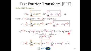
First, observe that the DFT sum involves complex exponentials e−j2πknN. We can split this sum into two parts: one for the even-indexed terms and one for the odd-indexed terms.
For N=2m, split the sequence x[n] into two subsequences:
● Even-indexed terms: x[0], x[2], x[4],…
● Odd-indexed terms: x[1], x[3], x[5],…
Let xeven[n]=x[2n] and xodd[n]=x[2n+1], and rewrite the DFT as:
X[k]=∑n=0N/2−1xeven[n]e−j2πkN(2n)+e−j2πkN∑n=0N/2−1xodd[n]e−j2πkN(2n).
This simplifies to:
X[k]=∑n=0N/2−1xeven[n]e−j2πkN(2n)+e−j2πkN∑n=0N/2−1xodd[n]e−j2πkN(2n).
By defining Xeven[k] and Xodd[k] as the DFTs of the even-indexed and odd-indexed subsequences, respectively, we get the following recursive relation:
X[k]=Xeven[k]+e−j2πkNXodd[k],
X[k+N/2]=Xeven[k]−e−j2πkNXodd[k].
Detailed Explanation
The first step of the Radix-2 Cooley-Tukey FFT algorithm involves breaking the Discrete Fourier Transform (DFT) into two parts—one for the even-indexed terms and another for the odd-indexed terms. By doing this, we define two new subsequences: 'even' for the terms at even indices (0, 2, 4...) and 'odd' for the terms at odd indices (1, 3, 5...). The sum of the DFT can then be expressed as two separate sums. This division reduces the complexity of the computation and lays the groundwork for a recursive computation. We can further simplify the expression by recognizing that the DFTs of the even and odd sequences can be computed recursively, leading to the formation of new relations that utilize previously calculated results. This is crucial because it allows us to break down the original DFT of size N into two smaller DFTs of size N/2.
Examples & Analogies
Imagine you have to analyze a large crowd at a concert. Instead of observing everyone at once, you split the crowd into two sections: left and right. First, you count how many people are standing on the left side, then you do the same for the right side. By only focusing on each section separately, you can manage your observations much more effectively. Similarly, in the Radix-2 FFT, by splitting the DFT into even and odd components, we can manage the computation more efficiently.
Step 2: Recursive Computation
Chapter 2 of 3
🔒 Unlock Audio Chapter
Sign up and enroll to access the full audio experience
Chapter Content
The process of splitting the DFT into smaller DFTs continues recursively until we reach the base case, where the DFTs are of size 2 (i.e., two-point DFTs). A two-point DFT is straightforward to compute:
X[0]=x[0]+x[1],
X[1]=x[0]−x[1].
This is the simplest form of the DFT, and it can be computed in constant time.
Detailed Explanation
After breaking the DFT into even and odd parts, the next step is to recursively apply the same strategy to these smaller DFTs. This recursive process continues until we reach the smallest possible DFTs—specifically, a DFT of size 2. The calculation of such small DFTs is extremely simple because it involves just two elements: you can find the two-point DFT by just adding and subtracting the two values. This reduction step is what makes the algorithm efficient, as it eventually leads to all DFTs being resolved back to their original size.
Examples & Analogies
Consider a family tree. Instead of trying to understand the entire family all at once, you start with the grandparents and divide them into two distinct branches: the mother's side and the father's side. You then repeat this process, breaking down each side into children, siblings, and eventually down to individual family members. By the time you get to the smallest unit (two siblings), you can easily understand their relationships. In FFT, we pursue a similar idea by recursively simplifying until we compute the simplest DFTs.
Step 3: Combining the Results
Chapter 3 of 3
🔒 Unlock Audio Chapter
Sign up and enroll to access the full audio experience
Chapter Content
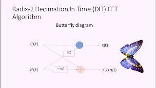
Once all the smaller DFTs are computed, the results are combined using the recursive formula:
X[k]=Xeven[k]+e−j2πkNXodd[k],
X[k+N/2]=Xeven[k]−e−j2πkNXodd[k].
The recursion terminates when the DFTs are computed for each pair of data points, and the final result is the DFT of the original sequence.
Detailed Explanation
The final step in the Radix-2 FFT algorithm is to combine the results obtained from the smaller DFT computations. Utilizing the recursive relationships established earlier, we can derive the DFT for the original sequence from the DFTs of the even and odd components. This process of recombining is carried out systematically until all DFT results are accumulated. At each stage, we make use of both addition and subtraction to merge these results appropriately using the defined formulas. Eventually, this leads us back to the complete DFT for the initial signal, completing the transformation.
Examples & Analogies
Think of assembling a large jigsaw puzzle. After you have pieced together various smaller sections (each representing small DFTs), you need to combine them into the larger picture. At the final stage, you carefully merge all the sections you've worked on until you create the full image. Similarly, once each segment of the DFT calculation is completed, they all come together to recreate the original signal's frequency information.
Key Concepts
-
Radix-2 FFT: A specific FFT algorithm that divides DFT into smaller DFTs, making computation efficient.
-
Recursion: A method where the algorithm calls itself to break down the problem into smaller pieces.
-
Twiddle Factor: A complex exponential factor used in the FFT computations, important for combining results.
Examples & Applications
The process of calculating the DFT of a sequence of twelve samples (e.g., N=12) using Radix-2 FFT involves breaking it into even and odd indexed samples, and recursively computing their DFTs.
If you had a time-domain signal represented by discrete samples, the Radix-2 FFT allows you to calculate its frequency components much faster than the standard DFT method.
Memory Aids
Interactive tools to help you remember key concepts
Rhymes
Even, odd, in pairs we split, to simplify and make it fit.
Stories
Imagine you are in a library organizing books. You can efficiently manage the books by first creating a section for every even-numbered book and another for the odd ones, making it easier to find the ones you need. This process is like how we organize the DFT in Radix-2 FFT!
Memory Tools
Recursion Cares: Break it down, solve the parts, combine at the end!
Acronyms
R.E.C.
Radix- Even/Odd
Combine - a quick way to remember the three steps of the FFT.
Flash Cards
Glossary
- DFT
Discrete Fourier Transform: A mathematical technique used to transform a sequence of values into frequencies.
- FFT
Fast Fourier Transform: An efficient algorithm to compute the DFT and its inverse.
- CooleyTukey
An algorithmic approach for efficiently computing the FFT by recursively breaking down DFTs.
- Twiddle Factor
Complex exponential factor used in the computation of FFT, represented as e^(-j2πkn/N).
- Recursive Relation
Mathematical relationship that allows computation of a function in terms of its values at smaller inputs.
Reference links
Supplementary resources to enhance your learning experience.