
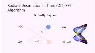
Step 3: Combining the Results
Interactive Audio Lesson
Listen to a student-teacher conversation explaining the topic in a relatable way.
Understanding the Combining Process
🔒 Unlock Audio Lesson
Sign up and enroll to listen to this audio lesson

Today, we will focus on the process of combining results in the Radix-2 FFT. This is crucial for understanding how we achieve the final DFT from smaller computations. Can anyone tell me what we've done so far before this step?

We broke down the DFT into even and odd parts!
Exactly! Now, we will use what we computed—two smaller DFTs—and start combining them using the formula: X[k] = X_even[k] + e^{-j 2πk/N} X_odd[k]. Can anyone explain what this formula tells us?

It shows how we combine the DFT of even parts with a phase shift from the odd parts.
Correct! The phase adjustment is crucial. Remember: regardless of whether it's even or odd, they both contribute to the final DFT. Let's repeat the key points. What do we achieve by combining these results?

We get the DFT of the original sequence efficiently!
Great! This efficiency is the heart of the Radix-2 FFT. The algorithm's ability to split and combine results allows us to reduce complexity significantly.
Understanding the Exponential Factors
🔒 Unlock Audio Lesson
Sign up and enroll to listen to this audio lesson

Now let's delve deeper into the exponential factor e^{-j 2πk/N}. Why do we adjust the odd-indexed results in this way?

Is it to account for the wave nature of the DFT? Like how the two parts are essentially the same but are at different phases?
Exactly! The phase adjustment ensures that we are accurately reflecting the periodic nature of the signals in our DFT. It’s like tuning into the right frequency. Can someone summarize why using the exponential factors is critical?
It ensures the correct combination of the real and imaginary parts from the even and odd calculations.
Well said! Each adjustment fine-tunes our final output, reflecting the true frequency content of our signal. Remember, these adjustments reduce computational errors and help compute the frequencies accurately.
Hands-on Application of the Concepts
🔒 Unlock Audio Lesson
Sign up and enroll to listen to this audio lesson
Let's apply our knowledge! If we have a small sequence of N = 4 where x = [1, 2, 3, 4], can someone remind me how we calculate the DFT of this sequence using the Radix-2 approach?
First, we split it into even and odd parts: [1, 3] and [2, 4].
Exactly! Now, compute the smaller DFTs for these parts. What do we get for X_even and X_odd?
X_even[0] = 1 + 3 = 4 and X_even[1] = 1 - 3 = -2. For X_odd, X_odd[0] = 2 + 4 = 6 and X_odd[1] = 2 - 4 = -2.
Perfect! Now use the combination formulas to compute the final result.
Using the formula, we have X[0] = 4 + e^{-j0} * 6 = 4 + 6 = 10 and X[1] = 4 - e^{-j0} * 6 = 4 - 6 = -2.
Nice job! You’ve just calculated the final DFT of our sequence using the Radix-2 FFT! This hands-on experience reinforces the theory we've discussed.
Introduction & Overview
Read summaries of the section's main ideas at different levels of detail.
Quick Overview
Standard
In this section, the focus is on how the Radix-2 FFT combines the results of smaller DFT computations, utilizing a recursive formula that helps to achieve efficient computation of the DFT. After breaking down the DFT into even and odd parts, this step illustrates how the results from these smaller parts are merged back together to yield the final DFT.
Detailed
Combining the Results in Radix-2 FFT
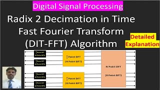
The Radix-2 FFT algorithm breaks down the Discrete Fourier Transform (DFT) into smaller, more manageable DFTs, reaching a foundation of two-point DFTs that can be computed directly. Once these smaller DFTs are calculated, the next critical step is combining the results to form the final output.
The combination occurs via the following equations:
- Combining Even and Odd Parts: Each element of the combined DFT is derived from the previously calculated DFTs of even and odd indexed parts.
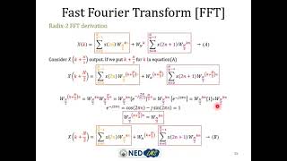
\[ X[k] = X_{even}[k] + e^{-j 2 \pi \frac{k}{N}} X_{odd}[k] \]
\[ X[k + N/2] = X_{even}[k] - e^{-j 2 \pi \frac{k}{N}} X_{odd}[k] \]
Here, \( X_{even}[k] \) and \( X_{odd}[k] \) are the DFTs computed from the even and odd subsequences, respectively. The exponential terms adjust the phase for the odd indexed terms based on their position in the composite DFT.
- Final Result: The recursive process continues until the combinations lead to the overall DFT of the original sequence. Thus the final output leverages the efficiencies created by breaking down the problem into simpler parts, affirming the power of the divide-and-conquer approach of the Radix-2 FFT.
This efficient combination step is what sets the Radix-2 FFT apart from direct computation methods, drastically reducing the operational complexity from O(N²) to O(N log N).
Youtube Videos
![Decimation In Time - Fast Fourier Transform [Lec 2]](https://img.youtube.com/vi/XeJXx-Te1Eo/mqdefault.jpg)
Audio Book
Dive deep into the subject with an immersive audiobook experience.
Combining the Smaller DFTs
Chapter 1 of 2
🔒 Unlock Audio Chapter
Sign up and enroll to access the full audio experience
Chapter Content
Once all the smaller DFTs are computed, the results are combined using the recursive formula:
X[k] = Xeven[k] + e^{- rac{j 2 \u03c0 k}{N}} Xodd[k]
X[k + N/2] = Xeven[k] - e^{- rac{j 2 c0 k}{N}} Xodd[k]
Detailed Explanation
In this chunk, we focus on how to combine the results of the smaller DFT computations into the final DFT result. We use the recursive formula to add together two components: the even-indexed part (Xeven[k]) and an adjusted version of the odd-indexed part (Xodd[k]) multiplied by a complex exponential factor. This combination derives from the original signal's structure and allows us to reconstruct the DFT of the entire sequence from its smaller parts. The second equation combines the results for the second half of the frequency bins, effectively giving us the full spectrum.
Examples & Analogies
Think of this process like putting together pieces of a jigsaw puzzle. Each smaller DFT acts like a smaller puzzle piece that contributes to the bigger picture (the complete DFT). By carefully aligning these pieces based on their connections (the even and odd parts), we can create a coherent image of the whole signal's frequency content.
Termination of Recursion
Chapter 2 of 2
🔒 Unlock Audio Chapter
Sign up and enroll to access the full audio experience
Chapter Content
The recursion terminates when the DFTs are computed for each pair of data points, and the final result is the DFT of the original sequence.
Detailed Explanation
Recursion involves calling a function within itself. In this context, it means that we continue breaking down the DFT into smaller DFTs until we reach the simplest units which are two-point DFTs. When these basic computations are completed, we start putting results back together, layer by layer, until the complete DFT of the original sequence is obtained. This organized way of combining results prevents errors and ensures accuracy in the final calculation.
Examples & Analogies
Imagine you are baking a multi-layer cake. You first bake each layer separately (the two-point DFTs) and then stack them one on top of the other (combining results from smaller DFTs). Just as you want each layer to fit perfectly and taste great together, you need to ensure that each computed part of the DFT fits together to accurately represent the whole signal.
Key Concepts
-
Combining Results: Refers to the process of merging small DFT results to compute the final DFT.
-
Exponential Factors: These adjustments ensure accurate phase representation in the final DFT results.
-
Recursive Formula: The relation defining how to combine even and odd parts of the DFT to arrive at the final output.
Examples & Applications
Using a sequence of numbers, we demonstrated how smaller DFTs are computed and then combined to get the DFT of the original sequence.
For N = 4, the sequence [1, 2, 3, 4] was split into [1, 3] and [2, 4]. The results from each were calculated and combined using the proper phase adjustments.
Memory Aids
Interactive tools to help you remember key concepts
Rhymes
When FFT we break apart, even-odd plays a vital part. Combine them, values turn bright, phase shifts bring them to light.
Stories
Imagine a baker splits the dough for cookie batches, some in even trays, some odd. After baking, he combines them for a delicious batch of treats—just as we combine DFT results for the sweet sound of frequencies!
Memory Tools
E-O-P: Even, Odd, Phase – helps me remember how to combine parts in FFT!
Acronyms
C.O.P (Combine Odd and Even Parts) is my guide for how to merge each part's DFT!
Flash Cards
Glossary
- Radix2 FFT
An efficient algorithm for computing the Discrete Fourier Transform (DFT) by recursively breaking it down into smaller DFTs.
- DFT
Discrete Fourier Transform, a mathematical transformation used to analyze the frequency content of discrete signals.
- Complex Exponential
A mathematical expression involving e raised to the power of an imaginary number, fundamental in Fourier analysis.
- Even and Odd Parts
The separation of a sequence into terms at even and odd indices, used to simplify the DFT calculation.
- Phase Adjustment
Changes made to the angles of frequencies during computations to ensure accurate representation in frequency domain.
Reference links
Supplementary resources to enhance your learning experience.