
Discrete Fourier Transform (DFT) Recap
Introduction & Overview
Read summaries of the section's main ideas at different levels of detail.
Quick Overview
Standard
The DFT facilitates the analysis of discrete signals by transforming them into the frequency domain through the use of complex exponential factors, but its direct computation is inefficient for large datasets due to its O(N²) complexity.
Detailed
Detailed Summary of Discrete Fourier Transform (DFT)
The Discrete Fourier Transform (DFT) is defined as:
$$X[k] = \sum_{n=0}^{N-1} x[n] e^{-j 2\pi \frac{kn}{N}} \text{where} \ k = 0, 1, \ldots, N-1$$
In this equation:
- $X[k]$ is the DFT of the time-domain signal $x[n]$ of length $N$.
- The term $e^{-j2\pi kn/N}$ is known as the complex exponential factor or the
Youtube Videos
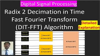
![Decimation In Time - Fast Fourier Transform [Lec 2]](https://img.youtube.com/vi/XeJXx-Te1Eo/mqdefault.jpg)
Audio Book
Dive deep into the subject with an immersive audiobook experience.
Definition of the DFT
Chapter 1 of 2
🔒 Unlock Audio Chapter
Sign up and enroll to access the full audio experience
Chapter Content
The Discrete Fourier Transform (DFT) of a sequence x[n] of length N is defined as:
X[k]=∑n=0N−1x[n]e−j2πknN for k=0,1,…,N−1
Where:
● X[k] is the DFT of x[n].
● x[n] is the time-domain signal of length N.
● e−j2πknN is the complex exponential factor (the "twiddle factor").
● k is the frequency index.
Detailed Explanation
The Discrete Fourier Transform (DFT) is a mathematical transformation used to analyze the frequency content of discrete signals. For a given sequence of values, the DFT converts it into a set of complex numbers, which represent the amplitude and phase of different frequency components within the original signal.
- Sequence Length: The input sequence
x[n]has a length ofN. - Output: The output
X[k]containsNvalues that correspond to different frequencies. - Complex Exponentials: The term
e^{-j2 ext{π}kn/N}is known as the twiddle factor, which helps in mixing the signal values to extract frequency information. - Frequency Index: The index
kranges from0toN-1, meaning we will getNfrequency components from our input signal.
Examples & Analogies
Think of the DFT like a baker who is creating a cake (the original signal). The various ingredients (individual values in the sequence x[n]) need to be analyzed to determine how they come together to create the cake's overall flavor (the frequencies captured by X[k]). The DFT helps the baker understand which ingredient contributes to which taste in the final product.
Direct Computation Complexity
Chapter 2 of 2
🔒 Unlock Audio Chapter
Sign up and enroll to access the full audio experience
Chapter Content
This direct computation of the DFT requires O(N2) operations, which becomes inefficient for large N.
Detailed Explanation
Computing the DFT directly involves summing an exponential term for each combination of signal values for every output frequency. This results in an operational complexity of O(N²), meaning that if we double the size of our input signal, the number of operations increases fourfold. As N grows larger, this inefficiency becomes a serious limitation, making it impractical for real-time applications or large datasets.
Examples & Analogies
Imagine a photographer who needs to take a team photo of a sports club with 200 members. If the photographer has to arrange each member for every possible lineup, the task becomes overwhelming quickly. The number of arrangements grows quadratically as more members are added. Just like the photographer would benefit from a more efficient way to set up the photo, processing large signals requires an efficient method to compute their DFT.