
Step 2: Recursive Computation
Interactive Audio Lesson
Listen to a student-teacher conversation explaining the topic in a relatable way.
Introduction to Recursive Computation
🔒 Unlock Audio Lesson
Sign up and enroll to listen to this audio lesson

Welcome class! Today we're diving deeper into the Recursive Computation step of the Radix-2 FFT. Can anyone explain what recursion means in this context?

Isn't recursion where a function calls itself to solve smaller instances of the problem?
Exactly! In the case of FFT, we're breaking the DFT into smaller DFTs recursively. Let's define the base case. Can anyone tell me what the base case is?

The base case happens when we reach two-point DFTs!
Correct! And what are those two-point DFT computations?

I think they're X[0] = x[0] + x[1] and X[1] = x[0] - x[1].
Great recall! By using these two-point computations, we can calculate larger DFTs quickly.
Let's remember this: recursion reduces complexity!
How Recursive Computation Works
🔒 Unlock Audio Lesson
Sign up and enroll to listen to this audio lesson

Now that we understand the base case, let's discuss how we continually divide the DFTs. Why do we split the DFT into even and odd parts?
To apply the Radix-2 FFT, right?
Correct! This helps us utilize the symmetry of the complex exponentials. What happens at the next level of recursion?

We keep dividing until we reach those two-point DFTs.
Exactly! This is what makes our calculations efficient. So, what happens to the computational time?
It goes from O(N²) to O(N log N)! That’s a huge reduction.
Well done! Now, let's summarize this process of continual halving for efficiency.
Significance of Recursive Computation in FFT
🔒 Unlock Audio Lesson
Sign up and enroll to listen to this audio lesson
Lastly, who can tell me why efficient computation is essential in real-world applications?
Because we handle large datasets! If calculations take too long, it’s impractical.
Exactly! The recursive approach of Radix-2 FFT allows us to analyze signals in real-time. What is an example of such an application?
Audio processing, like analyzing music frequencies!
Spot on! That’s how crucial our understanding of this recursion is. Let's keep in mind the core concepts discussed today as we progress.
Introduction & Overview
Read summaries of the section's main ideas at different levels of detail.
Quick Overview
Standard
In this section, we delve into the recursive computation of the Radix-2 FFT, illustrating how the DFT is broken down into smaller DFTs until a base case of two-point DFTs is reached. Here, we learn how these small computations lead to the efficient calculation of larger DFTs.
Detailed
Step 2: Recursive Computation
In the Radix-2 FFT algorithm, the process of computing the DFT is divided recursively into smaller computations. This section focuses on how this recursive division takes place and culminates in a straightforward computation of the simplest form of DFT, which consists of just two points.
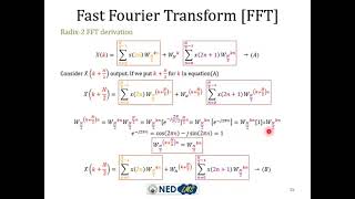
The recursive splitting continually breaks down a DFT of size N into DFTs of size N/2, continuing this process until reaching DFTs of size 2. At this base case of the computation, the two-point DFT is simply:
- X[0] = x[0] + x[1]
- X[1] = x[0] - x[1]
This approach allows each two-point DFT to be computed comfortably in constant time, making the entire FFT process efficient and manageable. Thus, the Radix-2 FFT elegantly reduces the complexity of DFT computation, paving the way for faster processing in applications involving large datasets.
Youtube Videos
![Decimation In Time - Fast Fourier Transform [Lec 2]](https://img.youtube.com/vi/XeJXx-Te1Eo/mqdefault.jpg)
Audio Book
Dive deep into the subject with an immersive audiobook experience.
Introduction to Recursive Computation
Chapter 1 of 2
🔒 Unlock Audio Chapter
Sign up and enroll to access the full audio experience
Chapter Content
The process of splitting the DFT into smaller DFTs continues recursively until we reach the base case, where the DFTs are of size 2 (i.e., two-point DFTs).
Detailed Explanation
In recursive computation, we repeatedly divide a problem into smaller sub-problems until we reach the simplest case, known as the base case. For the Radix-2 FFT algorithm, this base case occurs when we break down the Discrete Fourier Transform (DFT) into DFTs of size 2, which are easy to compute directly.
Examples & Analogies
Think of recursion like a fractal pattern in nature. Just like a tree branches into smaller sections, and those smaller sections can branch even further, the DFT is broken down into smaller DFTs, all the way down to the smallest possible size – which in this case are pairs of data points.
Computing the Two-Point DFT
Chapter 2 of 2
🔒 Unlock Audio Chapter
Sign up and enroll to access the full audio experience
Chapter Content
A two-point DFT is straightforward to compute:
X[0]=x[0]+x[1]
X[0] = x[0] + x[1]
X[1]=x[0]−x[1]
X[1] = x[0] - x[1]
Detailed Explanation
The two-point DFT involves only two data points, x[0] and x[1]. The computation is simple: we calculate the two frequency components based on these points. X[0] represents the sum of these points, while X[1] represents their difference. This simplicity makes it an ideal base case for our recursive algorithm.
Examples & Analogies
Imagine you are adding and subtracting two items from your shopping cart. If you buy two apples (x[0]) and one orange (x[1]), you can find the total number of fruits (X[0]) by adding them together, while finding the difference (X[1]) involves considering how many more apples you have compared to oranges.
Key Concepts
-
Recursive Computation: Breaking down the DFT into smaller DFTs recursively.
-
Base Case: The two-point DFT computation that serves as the simplest form for recursion.
-
Efficiency: The overall reduction of complexity from O(N²) to O(N log N) through recursive computation.
Examples & Applications
An example of the two-point DFT: X[0] = x[0] + x[1] and X[1] = x[0] - x[1].
Using larger datasets, we can recursively compute DFTs to analyze frequency components efficiently.
Memory Aids
Interactive tools to help you remember key concepts
Rhymes
To solve a DFT with ease, divide it down, if you please!
Stories
Imagine a baker who starts with one big cake and splits it into smaller layers until each piece is just right; that’s how we break down DFT!
Memory Tools
R-E-B: Recursive - Even and Odd - Base Case; helps remember the steps in computation.
Acronyms
A-B-C
Analyze
Break
Compute — the steps to recursively approach our DFT.
Flash Cards
Glossary
- Recursive Computation
The process of breaking down a problem into smaller instances of the same problem.
- Base Case
The simplest instance of a recursive function, which can be solved directly, such as a two-point DFT in this context.
- DFT
Discrete Fourier Transform, a mathematical transformation used to analyze the frequencies within a signal.
Reference links
Supplementary resources to enhance your learning experience.