
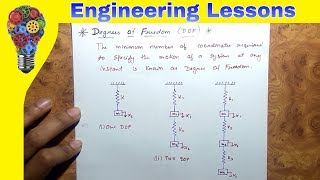
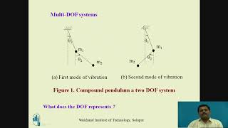
Damped 2-DOF Systems
Enroll to start learning
You’ve not yet enrolled in this course. Please enroll for free to listen to audio lessons, classroom podcasts and take practice test.
Interactive Audio Lesson
Listen to a student-teacher conversation explaining the topic in a relatable way.
Introduction to Damped 2-DOF Systems
🔒 Unlock Audio Lesson
Sign up and enroll to listen to this audio lesson

Today, we are discussing damped two-degree-of-freedom systems. Can anyone recall what the general equation of motion looks like for a damped system?

Isn't it Mx¨ + Cx˙ + Kx = 0?
That's correct! Now, what do you think the C matrix represents in this equation?

It represents the damping forces acting on the system?
Exactly! this accounts for the energy dissipation due to damping. And if we consider Rayleigh damping, how would the C matrix be expressed?

C = αM + βK, right?
Definitely! This form shows that damping is proportional to mass and stiffness matrices. These principles are crucial while assessing the behavior of structures.
Modal Transformation in Damped Systems
🔒 Unlock Audio Lesson
Sign up and enroll to listen to this audio lesson

Let’s dive into the concept of modal transformation. How does it change our analysis of a damped 2-DOF system?

It should uncouple the equations of motion, right? So, we can analyze each mode independently?
Absolutely! By transforming the displacement vector through modal coordinates, we get simpler equations to solve. Does anyone want to explain what these decoupled equations look like?
They would look like q¨ + 2ξωq˙ + ω²q = 0 for each mode?
Exactly! This uncoupling greatly simplifies the analysis for each mode, allowing us to understand the impact of damping on each vibrational mode individually.
Applications and Benefits of Damped 2-DOF Systems
🔒 Unlock Audio Lesson
Sign up and enroll to listen to this audio lesson
What do you think are some practical applications of understanding damped 2-DOF systems in our field?
I believe it helps in designing structures to resist vibrations during earthquakes.
Right! Considering the damping effects ensures that structures perform adequately under dynamic loads. How about the implications for tuning dampers?
Tuned mass dampers can be optimized using these analyses, limiting the structural response!
Excellent point! This knowledge is vital for enhancing earthquake resistance and ensuring structural integrity. Remember, assessing damping behavior is crucial for creating safer, more resilient buildings.
Introduction & Overview
Read summaries of the section's main ideas at different levels of detail.
Quick Overview
Standard
This section introduces damped 2-DOF systems by modifying the equations of motion to include damping, specifically exploring Rayleigh damping. The discussion highlights how modal transformation can still result in uncoupled equations, allowing for a simplified analysis of the system's dynamic response.
Detailed
In this section, we explore damped two-degree-of-freedom (2-DOF) systems, integral for understanding complex structures under dynamic loads. The overall equations of motion for a damped system are expressed as Mx¨ + Cx˙ + Kx = 0, where C represents the damping matrix. In cases where Rayleigh damping is applied, the damping matrix can be expressed as C = αM + βK, effectively making damped behavior proportional. We find that applying a modal transformation leads to decoupled equations, allowing for independent modal analysis of the damped system’s response. This simplifies the process of understanding how damping affects the dynamic behavior of structures subjected to various forces, important for practical applications in earthquake engineering.
Youtube Videos


Audio Book
Dive deep into the subject with an immersive audiobook experience.
Equations of Motion with Damping
Chapter 1 of 2
🔒 Unlock Audio Chapter
Sign up and enroll to access the full audio experience
Chapter Content
When damping is included, the equations of motion become:
Mx¨ + Cx˙ + Kx = 0
Where C is the damping matrix. If damping is proportional (Rayleigh damping):
C = αM + βK
Detailed Explanation
In this chunk, we see how the equations of motion change when damping is introduced to a two-degree-of-freedom system. The equation Mx¨ + Cx˙ + Kx = 0 describes the motion of the system, where M is the mass matrix, K is the stiffness matrix, and C is the damping matrix. The inclusion of the damping matrix (C) accounts for energy dissipation in the system, which is critical for realistic modeling of dynamic systems. The form of the damping matrix discussed, C = αM + βK, is known as Rayleigh damping, which suggests that the damping is a linear combination of the mass and stiffness matrices, where α and β are scalar constants that determine how much weight to give to each matrix in the damping calculation.
Examples & Analogies
Think of a swing in a playground. When you push the swing, it rises and falls (akin to the masses oscillating), but over time, if there’s any sort of friction (like air resistance or the rope rubbing on the swing set), the swing will eventually come to a stop. This friction represents damping in a mechanical system, dissipating energy and slowing down movement.
Decoupling of Equations
Chapter 2 of 2
🔒 Unlock Audio Chapter
Sign up and enroll to access the full audio experience
Chapter Content
Modal transformation still results in decoupled equations with damped response.
Detailed Explanation
Even with damping included, we can transform the system's equations into modal coordinates. This transformation helps us decouple the equations of motion, meaning that each equation can be solved independently. When systems are uncoupled, it simplifies our analysis because we can study the behavior of each mode separately instead of having to consider all modes at once. This decoupling is crucial as it allows engineers to understand the individual contributions of different vibrational modes to the overall response of the system.
Examples & Analogies
Consider a theater with multiple performances happening simultaneously. If each performer represents a different vibrational mode, decoupled equations would be like allowing each performer to practice their lines separately without interference from the others, making it easier to perfect their individual roles before coming together for the final show.
Key Concepts
-
Damping in 2-DOF Systems: The behavior of structures can be significantly influenced by energy dissipation, modeled through damping terms.
-
Rayleigh Damping: A specific formulation for damping that considers mass and stiffness contributions.
-
Modal Transformation: An essential technique which allows for the formulation of independent equations representing each mode of vibration.
Examples & Applications
A two-story building with floors considered as separate masses can be modeled as a damped 2-DOF system to assess its response during seismic activities.
In mechanical systems like vehicles, damped 2-DOF models can help analyze suspension systems under dynamic loading conditions.
Memory Aids
Interactive tools to help you remember key concepts
Rhymes
Damping adds a slowing sway, it stops the shudder, keeps at bay.
Stories
Imagine a bridge made of two beams wobbling during a windy day. When dampers are added, it distributes the shaking, making it safer and sound.
Memory Tools
Remember 'MCK' for Motion of a damped system: Mass, Couplings (K), and the damping matrix (C).
Acronyms
DAMP (Damping, Amplification, Modal Transformation, Proportional analysis) to remember the essentials of damped systems.
Flash Cards
Glossary
- Damped System
A dynamic system in which energy is lost over time due to the effect of damping forces.
- Rayleigh Damping
A type of damping that is proportional to both the mass and stiffness of the system.
- Modal Transformation
A technique used to transform the dynamic equations into uncoupled equations through modal coordinates.
Reference links
Supplementary resources to enhance your learning experience.