
MATLAB/Computational Implementation
Enroll to start learning
You’ve not yet enrolled in this course. Please enroll for free to listen to audio lessons, classroom podcasts and take practice test.
Interactive Audio Lesson
Listen to a student-teacher conversation explaining the topic in a relatable way.
Introduction to MATLAB for 2-DOF Systems
🔒 Unlock Audio Lesson
Sign up and enroll to listen to this audio lesson

Today, we'll explore how to implement the theory of 2-DOF systems using MATLAB. Can anyone tell me what a 2-DOF system is?

It's a system that requires two independent coordinates to describe its motion, like two masses connected by springs.
Exactly! Now, in MATLAB, we start by defining the mass and stiffness matrices. Who remembers what these matrices represent?

The mass matrix represents the inertial properties, while the stiffness matrix describes the system's resistance to deformation.
Good. Let’s look at how we define those in a MATLAB script.
Eigenvalue Problem in MATLAB
🔒 Unlock Audio Lesson
Sign up and enroll to listen to this audio lesson

Once we have our matrices, we use the ‘eig’ function to solve the eigenvalue problem. Can anyone recall the purpose of finding eigenvalues?

Eigenvalues give us the natural frequencies of the system, which are crucial for understanding vibration behavior.
Correct! The eigenvectors will then provide us with mode shapes. Now, let's see how that looks in MATLAB.

Can you show us an example of what the script should look like?
"Sure! Here's a basic example:
Plotting and Simulating Responses
🔒 Unlock Audio Lesson
Sign up and enroll to listen to this audio lesson
Visualizing results is key to understanding dynamics. How can we represent mode shapes in MATLAB?
We can use the ‘plot’ function to graph the mode shapes!
Exactly! After we compute the mode shapes, we can plot them to understand their spatial distribution. Let’s add that to our script.
What about simulating the system response to harmonic loads?
Good question! We can use the defined matrices to simulate how the system responds over time to different stimuli, like in earthquake loads.
Integration of Concepts
🔒 Unlock Audio Lesson
Sign up and enroll to listen to this audio lesson
Alright, let's summarize what we've learned. Can anyone outline the steps we need to analyze a 2-DOF system in MATLAB?
First, we define the mass and stiffness matrices, then solve the eigenvalue problem to find natural frequencies and mode shapes.
Then we plot the mode shapes and simulate the response.
Perfect! Integrating these ideas is crucial for practical earthquake engineering application.
Introduction & Overview
Read summaries of the section's main ideas at different levels of detail.
Quick Overview
Standard
The section outlines a general MATLAB script for analyzing 2-DOF systems. It covers the essential steps of defining mass and stiffness matrices, solving for natural frequencies and mode shapes, and simulating dynamic responses to various excitations.
Detailed
Detailed Summary
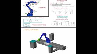
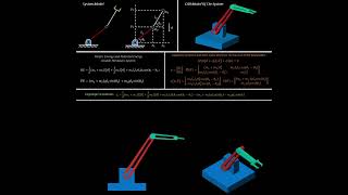
In engineering, computational tools like MATLAB play a crucial role in analyzing complex dynamic systems such as two-degree of freedom (2-DOF) models. This section illustrates the practical implementation of theory into computational scripts, highlighting key steps involved in the process. The MATLAB script typically includes the following steps:
1. Defining Mass and Stiffness Matrices: The first step is to define the mass (M) and stiffness (K) matrices that represent the physical properties of the 2-DOF system. In the given example, the matrices are defined as:
M = [1000 0; 0 1000];
K = [30000 -10000; -10000 30000];
- Solving for Eigenvalues and Eigenvectors: The script utilizes the
eigfunction to solve the eigenvalue problem, represented mathematically as \( K\Phi = \omega^2 M\Phi \). This helps in determining the natural frequencies \( \omega \) and mode shapes \( \Phi \). - Plotting Mode Shapes: Visualization is crucial in understanding the dynamic behavior. The script includes plotting commands to graphically represent the mode shapes.
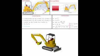
- Simulating System Response: Finally, the script allows for simulating the response of the 2-DOF system to harmonic or earthquake loads, enabling engineers to assess how the structure behaves under various conditions.
Understanding these computational implementations enriches the theoretical knowledge and prepares students for practical applications in earthquake engineering.
Youtube Videos


Audio Book
Dive deep into the subject with an immersive audiobook experience.
Introduction to MATLAB Implementation
Chapter 1 of 5
🔒 Unlock Audio Chapter
Sign up and enroll to access the full audio experience
Chapter Content
Most engineering analysis today involves computational tools. A typical MATLAB script for analyzing a 2-DOF system includes:
Detailed Explanation
This chunk introduces the context in which MATLAB is used for computational analysis in engineering. It mentions that modern engineering heavily relies on software tools like MATLAB for simulations and analysis instead of manual calculations.
Examples & Analogies
Think of it like cooking a recipe. Instead of preparing everything by hand, you might use a food processor to speed things up and ensure everything is mixed perfectly. Similarly, computational tools like MATLAB help engineers quickly analyze complex systems.
Defining Matrices M and K
Chapter 2 of 5
🔒 Unlock Audio Chapter
Sign up and enroll to access the full audio experience
Chapter Content
- Defining M,K
Detailed Explanation
In a MATLAB script, the first step is to define the mass matrix (M) and the stiffness matrix (K) for the 2-DOF system. These matrices represent the system's physical properties: M represents the mass distribution, and K defines how the system resists deformation.
Examples & Analogies
Imagine you are building a bridge. The mass matrix M represents the weight of the materials used (like steel and concrete), and the stiffness matrix K represents how strong the bridge is against bending and stretching. Just as these materials must be carefully chosen to ensure the bridge's safety, defining M and K accurately is crucial for a computer analysis.
Solving the Eigenvalue Problem
Chapter 3 of 5
🔒 Unlock Audio Chapter
Sign up and enroll to access the full audio experience
Chapter Content
- Solving the eigenvalue problem
Detailed Explanation
After defining the matrices, the next step is to solve the eigenvalue problem to find the natural frequencies and corresponding mode shapes of the 2-DOF system. In MATLAB, this involves using the 'eig' function, which computes eigenvalues and eigenvectors, providing information about how the system will respond to vibrations.
Examples & Analogies
This step can be likened to tuning a musical instrument. Just as a musician needs to know the correct pitches (frequencies) to tune their instrument properly, engineers need to determine the natural frequencies of a structure to ensure it performs well under stress.
Plotting Mode Shapes and Natural Frequencies
Chapter 4 of 5
🔒 Unlock Audio Chapter
Sign up and enroll to access the full audio experience
Chapter Content
- Plotting mode shapes and natural frequencies
Detailed Explanation
Once the eigenvalue problem is solved, the next step in the MATLAB script involves plotting the mode shapes and natural frequencies. This allows visual representation of how the system deforms during vibrational modes, which is essential for understanding the dynamic characteristics of the structure.
Examples & Analogies
This can be compared to visualizing how a trampoline moves when someone jumps on it. Observing the trampoline’s motion gives insight into how it reacts to weight changes. Similarly, by plotting mode shapes, engineers can see how a structure will behave when subjected to forces.
Simulating System Response
Chapter 5 of 5
🔒 Unlock Audio Chapter
Sign up and enroll to access the full audio experience
Chapter Content
- Simulating response to harmonic or earthquake base excitation
Detailed Explanation
The final step in the MATLAB script is to simulate how the system reacts to external forces, like harmonic excitations (regularly repeating forces) or earthquake movements. This simulation helps in analyzing the dynamic responses and assessing the safety and stability of the structure under different conditions.
Examples & Analogies
Consider a child on a swing being pushed — the way the swing moves in response to the pushes can be viewed as a simple model of how structures react to forces. Just as parents ensure swings are safe and stable, engineers use simulations to ensure structures can withstand forces like earthquakes.
Key Concepts
-
Mass and Stiffness Matrices: Essential matrices that define the physical properties of a 2-DOF system.
-
Eigenvalue Problem: A critical concept for determining frequencies and mode shapes of a dynamic system.
-
Mode Shape and Natural Frequency: Key outputs from the eigenvalue solution indicating the behavior of the system during vibrations.
Examples & Applications
Define a 2-DOF system with specified mass and stiffness parameters to analyze its dynamic behavior.
Use MATLAB scripts to visualize the mode shapes and simulate how the structure responds to different types of loads.
Memory Aids
Interactive tools to help you remember key concepts
Rhymes
For two degrees to understand, mass and stiffness go hand in hand.
Stories
Imagine two friends jumping on a trampoline; their movements depend on how heavy they are and how tightly the trampoline is stretched.
Memory Tools
Remember 'M' for Mass and 'K' for Kinetics to relate properties back to motions of systems.
Acronyms
2DOD
Two Degrees of Freedom Dynamics.
Flash Cards
Glossary
- Eigenvalue Problem
A mathematical problem that finds the natural frequencies and mode shapes of a system.
- Mass Matrix (M)
A matrix representing the mass distribution of the system.
- Stiffness Matrix (K)
A matrix representing the stiffness characteristics and resistance to deformation of the structure.
- Mode Shape
The spatial distribution of displacements in a system during a particular mode of vibration.
- Natural Frequency
The frequency at which a system tends to oscillate in the absence of external forces.
Reference links
Supplementary resources to enhance your learning experience.