
Equation Writing for Concentration Prediction
Enroll to start learning
You’ve not yet enrolled in this course. Please enroll for free to listen to audio lessons, classroom podcasts and take practice test.
Interactive Audio Lesson
Listen to a student-teacher conversation explaining the topic in a relatable way.
Introduction to Atmospheric Stability
🔒 Unlock Audio Lesson
Sign up and enroll to listen to this audio lesson

Today, we will explore the concept of atmospheric stability, which describes how air parcels behave in the atmosphere.

Why is atmospheric stability so important?
Great question! Stability affects how pollutants are transported. For instance, if a parcel is stable, it won’t rise as easily, and pollutants can accumulate.

What determines stability then?
Stability is determined by the temperature gradient. The adiabatic lapse rate we discussed means that temperature decreases with altitude. Understanding this helps us analyze different atmospheric conditions.

Can you remind us about the lapse rate?
Of course! The adiabatic lapse rate is approximately -0.0098 °C per meter. It’s a key factor when modeling air stability.
To summarize, atmospheric stability is crucial for predicting pollutant dispersion, determined by temperature gradients like the adiabatic lapse rate.
Mixing Height Concept
🔒 Unlock Audio Lesson
Sign up and enroll to listen to this audio lesson

Next, let's talk about mixing height. Can anyone explain what it is?

Isn’t it where the environmental lapse rate and adiabatic lapse rate meet?
Exactly! By defining mixing height, we can estimate the height at which pollutants can mix within the atmosphere.
What does this mean for pollutant plumes?
Good thinking! Mixing height affects how wide and dispersed a plume can become. The higher the mixing height, the more effectively pollutants can disperse.
To summarize, the mixing height concept is vital for predicting pollutant dispersion by determining how and where pollutants interact with the atmosphere.
Equation Development for Concentration Prediction
🔒 Unlock Audio Lesson
Sign up and enroll to listen to this audio lesson
Let's move on to writing equations for predicting pollutant concentrations. Who can point out what processes we need to consider?
Is it advection, dispersion, and reaction?
Correct! The equation we use for defining concentration accumulation includes these processes. Let’s denote the rate of accumulation as dC/dt.
How do we incorporate dispersion into the equation?
We use terms like rate in by dispersion and rate out by dispersion, related to Fick’s law. This takes us to the fundamental equation we discussed.
To wrap up, understanding how to write these equations allows us to quantitatively predict pollutant concentrations.
Fick's Law Application
🔒 Unlock Audio Lesson
Sign up and enroll to listen to this audio lesson
Now let’s apply Fick's Law to our pollutant dispersion model. Who remembers what Fick's Law represents?
It's about diffusion rates, right?
Exactly! It provides us with a way to describe how substances spread through a medium.
What’s the equation for it again?
The general form is J = -D (dC/dx), where J is the flux, and D is the diffusion coefficient. We’ll apply this in our dispersion equations.
In conclusion, Fick's Law is critical for modeling the diffusion aspect of pollutant dispersion.
Introduction & Overview
Read summaries of the section's main ideas at different levels of detail.
Quick Overview
Standard
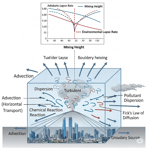
This section dives into the critical aspects of using box models for predicting pollutant concentrations in air, incorporating factors such as dispersion, advection, and atmospheric stability. It discusses the important processes affecting pollutant transport and provides insights on modeling these phenomena mathematically.
Detailed
Detailed Summary
This section addresses how to write equations that predict the concentration of pollutants in the air, using box models that focus on key transport processes. It first introduces the concept of stability in the atmosphere, essential for understanding how air parcels behave as they rise. The adiabatic lapse rate, defined as -0.0098 °C/m, is used to illustrate this stability. Furthermore, the potential temperature is introduced, which normalizes temperature for pressure variations.
The section outlines the mixing height concept, defined as the intersection of environmental lapse rate and adiabatic lapse rate, playing a crucial role in understanding plume behavior in pollutant dispersion. The governing equation for concentration prediction integrates various processes: advection, dispersion, and reaction, changing the concentration over time and space. Lastly, using Fick’s law of diffusion, a foundational equation is derived to model pollutant dispersion, emphasizing flow and dispersion rates.
Youtube Videos


Audio Book
Dive deep into the subject with an immersive audiobook experience.
Understanding the Control Volume
Chapter 1 of 4
🔒 Unlock Audio Chapter
Sign up and enroll to access the full audio experience
Chapter Content
So, last time when we were looking at the pollutant transport, our goal is to be able to predict concentration as function of place and time x, y, z and time. So, we look at one control volume within the plume, it is where the pollutant is moving and we try to model it.
Detailed Explanation
In this segment, the focus is on predicting the concentration of pollutants in the air as it moves through space and time (x, y, z coordinates along with time). A control volume is essentially a specific area we analyze, in this case, within the plume where pollutants accumulate. By observing this control volume, we can make estimations about the concentration of pollutants in this region based on their movement.
Examples & Analogies
Imagine monitoring the concentration of smoke in a room. You could consider a box (the control volume) within the smoke cloud to analyze how much smoke is in different parts of that box over time and space. This helps in understanding how smoke disperses within that area.
Writing the Accumulation Equation
Chapter 2 of 4
🔒 Unlock Audio Chapter
Sign up and enroll to access the full audio experience
Chapter Content
If you take this box which has dimensions of delta x, delta y, delta z, we have this term here rate of accumulation equals rate in by flow or rate out by flow, rate in by dispersion, rate out by dispersion.
Detailed Explanation
This part explains how to describe the behavior of pollutants mathematically within the control volume. The 'rate of accumulation' refers to the amount of pollutant that builds up in the control volume over time. This can be influenced by several factors: the rate at which pollutants enter (in by flow), leave (out by flow), and diffuse (in by dispersion and out by dispersion). By equating these rates, we can create a balanced equation that captures the dynamics of the pollutant concentration.
Examples & Analogies
Think of a bathtub filling with water. The rate of water coming in through the tap represents the 'rate in by flow,' while the rate draining out represents 'rate out by flow.' Similarly, if you spill some water (dispersion), it changes the amount accumulating in the tub. By understanding these rates, you can predict how full your tub will be after a certain time.
Identifying Processes in the Transport Model
Chapter 3 of 4
🔒 Unlock Audio Chapter
Sign up and enroll to access the full audio experience
Chapter Content
So, the transport model can have anything the generalized transport model will also have a reaction, will also have adsorption, will also have deposition all these things will happen this multi-phase model but we are not doing that here we are looking at only C, so C is vapor phase concentration only.
Detailed Explanation
Here, the discussion shifts to the processes involved in the pollutant transport model. A generalized transport model may include various processes such as reactions (chemical changes), adsorption (pollutant particles sticking to surfaces), and deposition (settling out of the air). However, the focus in this context is solely on vapor phase concentration (C), which simplifies the analysis to one specific aspect of the model.
Examples & Analogies
Imagine making a smoothie. The fruits (the pollutants) can blend well (vapor phase concentration), react with each other (react), stick to the blender walls (adsorption), or settle at the bottom (deposition). If we're only interested in the blended part of the smoothie (vapor concentration), we ignore what happens to the fruits outside the blender.
Predicting Exposure Concentration
Chapter 4 of 4
🔒 Unlock Audio Chapter
Sign up and enroll to access the full audio experience
Chapter Content
So, in this case, we are writing it for this particular A in the phase that we are interested in, the vapor phase only because this is the phase we are interested in calculating exposure at some point.
Detailed Explanation
This chunk emphasizes the specific focus of the concentration predictions on the vapor phase of pollutants. Measuring this phase is crucial for understanding potential exposure to individuals nearby. By concentrating solely on the vapor concentration of pollutant A, we can determine how much of it a person might be exposed to based on their location and the plume's behavior.
Examples & Analogies
Think of standing next to a campfire where smoke is rising. The vapor phase is like the smoke that you can smell and breathe. If you're interested in how much smoke (pollutant A) enters your lungs, you would monitor only the smoke in the air around you rather than what’s left behind on the ground after the fire is out.
Key Concepts
-
Atmospheric Stability: Refers to how air parcels behave in the atmosphere, affecting pollution dispersion.
-
Adiabatic Lapse Rate: The constant rate of temperature decrease with altitude in a rising air parcel, essential for modeling stability.
-
Mixing Height: The intersection of environmental and adiabatic lapse rates where pollutant mixing occurs.
-
Concentration Prediction: The process of modeling how pollutants disperse in the atmosphere using specific equations.
-
Fick's Law of Diffusion: A fundamental law governing the spread of particles in a medium based on concentration differences.
Examples & Applications
Example of measuring mixing height to assess the dispersion potential of a pollutant release.
Application of Fick's Law to determine the concentration gradient of a contaminant in a controlled environment.
Memory Aids
Interactive tools to help you remember key concepts
Rhymes
When air is high, it's cold and shy; Stability drops when the warmth does fly.
Stories
Imagine a hot air balloon rising. As it climbs, it cools down. If it cools too much, it doesn't rise effectively, illustrating atmospheric stability.
Memory Tools
To remember Fick's Law: 'Flux Favors Fast Flow'. This points to how flux is driven by concentration differences.
Acronyms
M.A.P. for Mixing, Adiabatic, Potential - the three key concepts in understanding air stability and pollutant dispersion.
Flash Cards
Glossary
- Adiabatic Lapse Rate
The rate of temperature decrease with an increase in altitude in a rising air parcel, approximately -0.0098 °C/m.
- Mixing Height
The height in the atmosphere where the environmental lapse rate intersects with the adiabatic lapse rate, impacting pollutant dispersion.
- Dispersion
The process through which pollutants spread out into the atmosphere, influenced by various physical forces.
- Fick's Law
A principle that describes the diffusion flux of particles within a medium based on concentration gradients.
- Potential Temperature
The temperature of an air parcel corrected to a standard pressure, typically sea level pressure.
Reference links
Supplementary resources to enhance your learning experience.