
Rate of Flow and Dispersion
Enroll to start learning
You’ve not yet enrolled in this course. Please enroll for free to listen to audio lessons, classroom podcasts and take practice test.
Interactive Audio Lesson
Listen to a student-teacher conversation explaining the topic in a relatable way.
Understanding Mixing Height
🔒 Unlock Audio Lesson
Sign up and enroll to listen to this audio lesson

Today, we will start by understanding what mixing height means. Can anyone tell me why mixing height is important?

Isn't it about how pollutants mix in the air?
Exactly! Mixing height is the altitude at which pollutants effectively disperse. It depends on atmospheric stability. What do you think affects stability?

Temperature, right? The air temperature gradient?
That's right! The interaction of the air parcel’s temperature with the surrounding atmosphere plays a crucial role. Remember, the term 'adiabatic lapse rate' describes this temperature change as height increases. Can anyone tell me the value of the dry adiabatic lapse rate?

Isn’t it -0.0098 °C per meter?
Correct! Now, let's reflect on how mixing height can influence air quality.

How does it affect pollution concentration?
Good question! A higher mixing height can dilute pollutants, leading to lower concentrations at ground level. Let’s summarize: mixing height is influenced by stability and temperature gradients, crucial for pollution dispersion.
Dispersion Modeling
🔒 Unlock Audio Lesson
Sign up and enroll to listen to this audio lesson

Now let’s dive into dispersion modeling. Why do we need equations to model pollution dispersion?
To predict how pollutants spread in the air?
Precisely! We use a control volume to help us. We’ll denote it as a box filled with pollutants. What key processes do we consider for pollution transfer?
Advection and dispersion?
Exactly! We focus on the rates of accumulation and flow. The equation typically looks like the rate of accumulation equals rate of flow in minus rate of flow out. Can anyone think of other processes that might affect this model?
Chemical reactions and deposition?
Exactly! But for our simplified model, we will assume no reactions are occurring for now. Understanding these concepts enables us to predict the concentration of pollutants over time.
What about the flux term in this equation?
Great question! The flux term is derived from Fick's law of diffusion, representing how substances disperse through space. Let's summarize: pollution modeling involves flow rates and mass balance, vital for predictions!
Applications and Importance of Modeling
🔒 Unlock Audio Lesson
Sign up and enroll to listen to this audio lesson
Having discussed the theory, why do you think understanding dispersion models is important?
To help predict environmental impacts and regulatory standards?
Yes! Models can help advise urban planning and monitor air quality compliance. For example, estimating pollutant exposure for people living near emission sources is vital. What methods can we use to validate our models?
Collecting real-time air quality data?
Exactly! By comparing expected concentrations from our models with actual measurements, we can refine our predictions. Let's wrap up by summarizing the key points we’ve discussed: the importance of dispersion modeling in understanding air quality.
Introduction & Overview
Read summaries of the section's main ideas at different levels of detail.
Quick Overview
Standard
The section examines how pollutants disperse in air through advection, stability, and mixing height. It discusses critical terms like adiabatic lapse rate and potential temperature, which affect pollutant behavior, and outlines the modeling of these processes using mass balance equations.
Detailed
Detailed Summary of Rate of Flow and Dispersion
This section discusses the importance of understanding air dispersion processes for effective monitoring and analysis of environmental quality. Core to this understanding is the concept of mixing height, which is influenced by atmospheric stability. Stability is defined in terms of temperature gradients and the behavior of air parcels as they rise.
Key highlights include:
- The adiabatic lapse rate, which is specified as -0.0098 °C/meters, indicating how temperature decreases with altitude in an adiabatic process.
- Potential temperature (θ) as a normalized temperature reflecting air parcel behaviors at varying pressures.
- The definition of mixing height and its significance in identifying where dispersion processes occur.
- The mathematical representation of pollutant dispersion, featuring advection and Fick’s law, highlighting rates of flow in one-dimensional and three-dimensional models.
- Utilizing control volumes and establishing mass balance equations to model concentration predictions over time and space, ensuring that environmental impacts of pollutants can be assessed accurately.
Youtube Videos


Audio Book
Dive deep into the subject with an immersive audiobook experience.
Introduction to Box Models
Chapter 1 of 7
🔒 Unlock Audio Chapter
Sign up and enroll to access the full audio experience
Chapter Content
So, we were looking at box models for pollutant transfers in air. So, essentially this is a generic box model for air. The processes that we are considering in the box include advection, dispersion, reaction exchange, and all that, ok.
Detailed Explanation
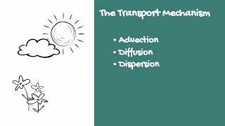
In environmental science, we use box models to understand how pollutants are transferred in the atmosphere. A box model simplifies a complex system by treating it as a box (or container) that holds air and pollutants. The box allows us to study various processes such as advection (the horizontal movement of air), dispersion (how pollutants spread out), and reactions (how pollutants interact with one another) within the air.
Examples & Analogies
Imagine a fish tank where you drop a few drops of food coloring. The color spreads out due to the movement of water (advection) and the mixing of the water (dispersion). This helps us visualize how pollutants will behave in the air.
Understanding Atmospheric Stability
Chapter 2 of 7
🔒 Unlock Audio Chapter
Sign up and enroll to access the full audio experience
Chapter Content
So, the specific problem for air is that the height is not very well defined, so we look at what is called as a mixing height and mixing height depends on concept called stability and stability is function of temperature in the lower atmosphere.
Detailed Explanation
The concept of mixing height is critical in understanding how pollutants disperse in the atmosphere. Mixing height refers to the vertical distance in the air where pollutants are mixed effectively. It's influenced by atmospheric stability, which is a measure of how temperature affects the vertical movement of air parcels. A stable atmosphere means less vertical movement, while an unstable atmosphere allows pollutants to rise and disperse more easily.
Examples & Analogies
Think of making a soup. If the soup is hot (unstable), steam rises and mixes with the air, making it more aromatic. If the soup is cold (stable), the steam doesn't rise much, and the aromas stay trapped, similar to how pollutants behave under stable atmospheric conditions.
Adiabatic Lapse Rate
Chapter 3 of 7
🔒 Unlock Audio Chapter
Sign up and enroll to access the full audio experience
Chapter Content
The lapse rate represented by Gamma, the adiabatic lapse rate is given as -0.0098 centigrade per kilo per meter or 9.8 centigrade per kilometer this is the adiabatic lapse rate.
Detailed Explanation
The adiabatic lapse rate describes how temperature changes with altitude in a rising air parcel. Specifically, it states that as an air parcel rises, it cools at a consistent rate of about 9.8 degrees Celsius for every kilometer it ascends. This cooling occurs because the air parcel expands and does work against the surrounding atmosphere without exchanging heat, known as an adiabatic process.
Examples & Analogies
When you go hiking and climb a mountain, you might notice it gets colder as you go up. This is due to the adiabatic lapse rate affecting the temperature of the air around you. Your experience simulates how temperature drops with elevation.
Potential Temperature
Chapter 4 of 7
🔒 Unlock Audio Chapter
Sign up and enroll to access the full audio experience
Chapter Content
There is another term called potential temperature is defined like this theta equals T0, this is the temperature corrected to particular pressure, so the pressure with reference to sea level pressure.
Detailed Explanation
Potential temperature is a useful concept in meteorology that refers to the temperature an air parcel would have if there were no changes in pressure as it moved. It allows us to compare air parcels at different altitudes and pressures by normalizing their temperatures to sea level. Understanding potential temperature helps in analyzing stability and predicting the vertical movement of air masses.
Examples & Analogies
Consider a balloon filled with air. As the balloon ascends, the pressure inside it decreases, and the air cools. If we could measure its temperature if it were brought back to the ground without changing the pressure, that would be its potential temperature.
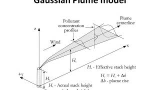
Mixing Height and Plume Formation
Chapter 5 of 7
🔒 Unlock Audio Chapter
Sign up and enroll to access the full audio experience
Chapter Content
We also looked at this concept of mixing height, mean mixing height as the place where the intersection of the environmental lapse rate and adiabatic lapse rate happens.
Detailed Explanation
Mixing height is critical for understanding where pollutants will disperse in the atmosphere. It corresponds to the height where the environmental lapse rate (actual temperature gradient in the atmosphere) meets the adiabatic lapse rate. This height defines the top of the layer where pollutants are efficiently mixed and can impact air quality at ground level.
Examples & Analogies
Think of a layer of bread in a toaster: the top layer receives more heat (mixing height) and rises as it cooks, while the lower layers (below the mixing height) might stay cooler. Similarly, pollutants disperse as they reach the mixing height before stabilizing.
Predicting Pollutant Concentration
Chapter 6 of 7
🔒 Unlock Audio Chapter
Sign up and enroll to access the full audio experience
Chapter Content
So, our goal is to be able to predict concentration as a function of place and time x, y, z and time.
Detailed Explanation
The ultimate goal in studying air quality is to predict how pollutant concentrations will vary depending on location (x, y, z coordinates) and time. By modeling these changes, we can understand how and where pollutants will affect different areas, helping us design better strategies to manage air quality and minimize health risks.
Examples & Analogies
Imagine forecasting the spread of wildfire smoke. Just like meteorologists predict how smoke will move and settle in certain areas based on wind patterns and geographical features, scientists use similar models to predict pollution spread.
Equations for Accumulation and Dispersion
Chapter 7 of 7
🔒 Unlock Audio Chapter
Sign up and enroll to access the full audio experience
Chapter Content
So, if you take this box which has dimensions of delta x, delta y, delta z, we have this term here rate of accumulation equals rate of in by flow or rate out by flow, rate in by dispersion, rate out by dispersion.
Detailed Explanation
The equations used in box models calculate the rates of accumulation of pollutants. They consider how pollutants flow in and out of a defined volume (the box) and the dispersion within that volume. Essentially, these equations help us quantify how much pollution enters or leaves a certain area over time, allowing us to assess air quality better.
Examples & Analogies
Think of a bathtub being filled with water. The rate at which water flows in (inflow) and out (outflow), as well as how it spreads around (dispersion), determines how full the tub gets. Similarly, understanding these rates helps us see how pollution levels change over time.
Key Concepts
-
Mixing Height: The altitude at which air pollutants disperse effectively depends on atmospheric conditions.
-
Adiabatic Lapse Rate: A standard for understanding how temperature varies with altitude in the absence of heat transfer.
-
Potential Temperature: A useful method for normalizing temperature data for pressure variations.
Examples & Applications
A tall smokestack releases pollutants that disperse more effectively at higher mixing heights, leading to lower concentrations at ground level.
In a thermal inversion scenario, stable atmospheric conditions prevent pollutants from dispersing, leading to higher ground-level concentrations.
Memory Aids
Interactive tools to help you remember key concepts
Rhymes
When air goes high, temperatures drop, mixing height helps pollutants stop.
Stories
Imagine a balloon rising, carrying colorful smoke. At the top, the smoke spreads wide, while at the bottom, it stays confined. This represents mixing height.
Memory Tools
MOLD: Mixing height, Oxygen levels, Lapse rates, Dispersion processes—all are key.
Acronyms
M.A.P.
Mixing height
Adiabatic lapse rate
Potential temperature—guides for dispersion.
Flash Cards
Glossary
- Adiabatic Lapse Rate
The rate at which an air parcel cools as it rises in the atmosphere, approximately -0.0098 °C/meter.
- Mixing Height
The altitude at which pollutants effectively disperse in the atmosphere.
- Potential Temperature
The temperature of an air parcel adjusted to a standard reference pressure, typically sea-level pressure.
- Dispersion
The process by which pollutants spread through air or water due to various forces.
- Advection
The horizontal transfer of pollutants through wind or water currents.
Reference links
Supplementary resources to enhance your learning experience.