
Shape of Plumes
Enroll to start learning
You’ve not yet enrolled in this course. Please enroll for free to listen to audio lessons, classroom podcasts and take practice test.
Interactive Audio Lesson
Listen to a student-teacher conversation explaining the topic in a relatable way.
Understanding Mixing Height and Stability
🔒 Unlock Audio Lesson
Sign up and enroll to listen to this audio lesson

Let's start with the mixing height. Mixing height is crucial for understanding how pollutants disperse in the atmosphere. What factors influence mixing height?

Is it affected by temperature?
Exactly! The mixing height is influenced by temperature and stability in the atmosphere. Stability refers to how an air parcel behaves as it rises. Can anyone tell me what adiabatic expansion is?

Isn't it when the air parcel cools as it rises?
That's right! As the air parcel rises, it expands adiabatically, leading to cooling. This cooling is described by the adiabatic lapse rate, which is about -0.0098 °C per meter or 9.8 °C per kilometer. Remember: 'higher rises, cooler surprises!'

How does this lapse rate relate to mixing height?
Great question! The mixing height is where the adiabatic lapse rate meets the environmental lapse rate. This intersection is critical for predicting where pollutants might be effectively dispersed.

So it's all about the stability of the atmosphere!
That's right! Remember, understanding how stability influences mixing height helps us predict pollutant behavior.
Exploring Plume Shapes
🔒 Unlock Audio Lesson
Sign up and enroll to listen to this audio lesson

Now, let's discuss plume shapes. How many different plume shapes can you think of based on environmental conditions?
I think there are a few like the linear plume or the Gaussian shape?
Exactly! There are various forms of plumes based on combinations of factors like source height and stability conditions. Can you guess why knowing these shapes is important?
Maybe to predict where pollutants will travel?
Precisely! Predicting pollutant dispersal helps assess air quality and potential human exposure. The time-averaged shape of a plume gives us essential data for these predictions.
What happens if the source height is much taller?
Good observation! Taller sources can lead to higher plumes, which disperse pollutants over a larger area. Always remember: 'height helps flight!'
So every situation can create a unique plume shape!
That's correct! Understanding the fundamentals of plume shape lets us predict their behavior in various environmental contexts.
Transport Model Dynamics
🔒 Unlock Audio Lesson
Sign up and enroll to listen to this audio lesson
To model pollutants, we must consider transport dynamics. What do you think are the main processes we should include in our model?
I think we should include advection and dispersion?
Correct! Advection and dispersion, along with reaction and deposition, are key processes. Let's focus on advection first. What do you understand by advection?
It’s when pollutants are carried away by wind?
Exactly! Advection helps in the horizontal movement of pollutants. Now, let’s define dispersion within our context. What is dispersion?
It’s the spreading out of pollutants, right?
That’s right! Dispersion often results from factors like buoyancy and wind. Together, advection and dispersion create complex pollutant plumes! Remember: 'advection drives direction, dispersion creates diffusion!'
How do we model these processes mathematically?
We use conservation equations that balance the inflow and outflow of pollutants in a defined volume—often framed in terms of rates of accumulation.
Introduction & Overview
Read summaries of the section's main ideas at different levels of detail.
Quick Overview
Standard
In this section, we delve into the intricacies of air pollutant dispersion through the prism of box models. We explore key concepts such as environmental stability, mixing height, and how these factors influence the shape of pollutant plumes, helping in understanding their dispersion in air over time and spatial dimensions.
Detailed
Detailed Summary
In the study of atmospheric dispersion, understanding the behavior and shape of pollutant plumes is crucial. This section explores the concept of mixing height, which is influenced by the atmospheric stability that in turn is a function of temperature differentials in the lower atmosphere. The ideal adiabatic expansion behavior of air parcels is explained, complemented by terms such as the environmental lapse rate, which represents changes in temperature with altitude.
The section discusses the dry adiabatic lapse rate determined as -0.0098°C per meter, a constant that holds under conditions of adiabatic processes without heat transfer. Additionally, potential temperature is introduced as a normalized temperature adjustment based on atmospheric pressure, illustrating how it helps to analyze thermal stratification.
The interactions between the environmental lapse rate and the dry adiabatic lapse rate define mixing height, the critical altitude where pollutants disperse most effectively. Various plume shapes arise depending on these environmental conditions, enabling predictions about the dispersion behavior of pollutants emitted into the atmosphere. The section concludes with the formulation of a transport model encompassing rates of flows and dispersion processes within environmental contexts.
Youtube Videos


Audio Book
Dive deep into the subject with an immersive audiobook experience.
Mixing Height and Atmospheric Stability
Chapter 1 of 4
🔒 Unlock Audio Chapter
Sign up and enroll to access the full audio experience
Chapter Content
And we also looked at this concept of mixing height, mean mixing height as the place where the intersection of the environmental lapse rate and adiabatic lapse rate happens.
Detailed Explanation
Mixing height is a crucial concept for understanding how pollutants travel in the air. It is defined as the altitude where the environmental lapse rate (the rate at which temperature decreases with altitude in the atmosphere) intersects with the adiabatic lapse rate (the rate at which a parcel of air cools as it rises). The mixing height indicates the vertical extent of the atmosphere where mixing occurs due to turbulence, which is important for dispersion of pollutants.
Examples & Analogies
Imagine cooking in a pot of boiling water. The steam represents pollutants rising into the air. The top of the pot's steam indicates the mixing height, where the steam can spread out into the room. If the kitchen is well ventilated (like a stable atmosphere), the steam disperses quickly, while in a closed kitchen (like an unstable atmosphere), the steam might condense and linger.
Understanding Plume Shape
Chapter 2 of 4
🔒 Unlock Audio Chapter
Sign up and enroll to access the full audio experience
Chapter Content
And we also defined that this is the plume the boundary of this thing so you can say within this a lot of things happen plume may go in and out but there is something called as a time averaged plume.
Detailed Explanation
A plume is the visible or measurable part of the emitted pollutants as they disperse in the atmosphere. The 'shape' of a plume refers to how it spreads out in the air over time and in space. The time-averaged plume is a representation of what happens when pollutants are emitted over a period. It helps scientists understand typical dispersion patterns and predict the impact of pollutants on air quality.
Examples & Analogies
Think of a plume like smoke from a campfire. When the fire burns steadily, the smoke rises and spreads out in a specific shape, creating a 'cloud' of smoke. If the wind blows, the shape shifts and stretches. Over time, if we observe the smoke from different angles and occasions, we can begin to predict its usual shape and how far it would spread.
Factors Affecting Plume Shape
Chapter 3 of 4
🔒 Unlock Audio Chapter
Sign up and enroll to access the full audio experience
Chapter Content
So this is one set of conditions, but if you know the basic fundamental aspects behind it you can predict what is the kind of plume shape that you can expect for a given situation.
Detailed Explanation
The specific shape of a plume is influenced by several factors, including the height of the emission source, the dispersion conditions like temperature and wind, and the stability of the atmosphere. Understanding these factors allows us to model and predict the expected behavior of a pollutant plume more accurately in different environmental scenarios.
Examples & Analogies
Consider pouring a drop of dye into a still glass of water and then into a glass of water that’s being stirred. In the still water (stable atmosphere), the dye forms a small localized patch. In the stirred water (unstable), the dye disperses quickly and broadly, forming different shapes based on how vigorously the water is mixed. Just like with smoke or pollutants, the activity around the source significantly changes how dispersion occurs.
Pollutant Transport and Concentration Prediction
Chapter 4 of 4
🔒 Unlock Audio Chapter
Sign up and enroll to access the full audio experience
Chapter Content
So last time when we were looking at the pollutant transport, our goal is to be able to predict concentration as a function of place and time x, y, z and time.
Detailed Explanation
In studies of air pollution, one primary goal is to predict how pollutants will concentrate in various locations over time. This involves modeling the dispersion of pollutants in a three-dimensional space (x, y, z) and considering how concentrations change. By understanding plume shape and the dynamics of the atmosphere, scientists can create models that estimate pollutant concentrations at different points around the emission sources.
Examples & Analogies
Imagine you're at a music concert. The sound from the speakers (pollutants) spreads out into the area (3D space), but how loud it is (concentration) varies depending on where you are standing relative to the speakers. Some areas close to the speakers may be very loud (high concentration), while areas further away may hear much less sound (lower concentration). Predicting noise levels in different spots is similar to modeling pollutant concentrations.
Key Concepts
-
Mixing Height: The altitude crucial for pollutant dispersion, where environmental and adiabatic lapse rates meet.
-
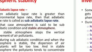
Stability: Refers to the behavior of air parcels influenced by temperature gradients, impacting the dispersion of pollutants.
-
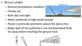
Plume Shapes: Different forms of pollutant plumes determined by environmental conditions, source height, and atmospheric stability.
-
Advection and Dispersion: Key atmospheric processes that dictate how pollutants move in space and time.
Examples & Applications
Example of a linear plume observed above a factory emitting pollutants into the atmosphere.
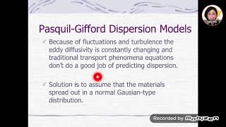
A Gaussian plume model illustrating how pollutants spread under stable atmospheric conditions.
Memory Aids
Interactive tools to help you remember key concepts
Rhymes
Higher the plume, cooler the air; stability drives how pollutants fare.
Stories
Imagine a rising balloon, as it goes higher, it cools down and expands, illustrating how smoke from a chimney behaves while dispersing in the air.
Memory Tools
Remember the acronym 'MAPS' for mixing height—Mixing, Adiabatic, Potential temperature, Stability.
Acronyms
Use the acronym 'PEAR' to recall key processes
Pollutants
Environmental Lapse rate
Advection
and Reactions.
Flash Cards
Glossary
- Mixing Height
The altitude at which the environmental lapse rate meets the adiabatic lapse rate; crucial for pollutant dispersion.
- Stability
The behavior of an air parcel as it rises or falls in the atmosphere, dictated by temperature gradients.
- Adiabatic Lapse Rate
Rate at which temperature decreases with height in a rising air parcel, typically at -0.0098°C per meter.
- Potential Temperature
The temperature of an air parcel if brought to a reference pressure, aiding in determining stability.
- Advection
The horizontal transport of pollutants due to wind.
- Dispersion
The spreading of pollutants in the atmosphere due to various effects like buoyancy and turbulence.
Reference links
Supplementary resources to enhance your learning experience.