
Lecture-39
Enroll to start learning
You’ve not yet enrolled in this course. Please enroll for free to listen to audio lessons, classroom podcasts and take practice test.
Interactive Audio Lesson
Listen to a student-teacher conversation explaining the topic in a relatable way.
Understanding Mixing Height
🔒 Unlock Audio Lesson
Sign up and enroll to listen to this audio lesson

Today, let's discuss mixing height, which is crucial in understanding how pollutants disperse in the air. Can anyone tell me why mixing height is significant?

It's important because it determines the altitude at which pollutants can mix with the atmosphere.
Exactly! Mixing height refers to the height in the atmosphere where pollutants and air mix effectively. It depends on atmospheric stability. What do we mean by atmospheric stability?

It defines how a parcel of air behaves as it rises, mainly depending on temperature.
Correct! Remember, stability is affected by the environmental lapse rate—a very important concept. Let's use the acronym 'SHEAR' to remember Stability, Height, Environmental lapse rate, Adiabatic lapse, and Reaction.

But what is the adiabatic lapse rate again?
Great question! The adiabatic lapse rate is approximately -0.0098 °C/m. It describes the temperature change of an ascending air parcel under adiabatic conditions!

So it doesn’t change based on where it’s emitted?
Exactly! The lapse rate remains constant regardless of the emission source.
Let’s summarize: Mixing height is crucial for pollutant dispersion as influenced by atmospheric stability, and you should remember the acronym 'SHEAR' when studying.
Potential Temperature and Its Importance
🔒 Unlock Audio Lesson
Sign up and enroll to listen to this audio lesson

Now, let’s talk about potential temperature. Can anyone explain what it is?
It’s the temperature of an air parcel corrected for pressure, right?
Exactly! When an air parcel rises, its temperature changes with pressure, and potential temperature accounts for that change. Why is this important in atmospheric studies?
It helps in determining stability and inversion layers in the atmosphere.
Well said! Remember, potential temperature allows us to normalize temperature data for better comparisons.
How do we calculate potential temperature?
We use the formula, θ = T0, where T0 is the temperature corrected for a reference pressure. It’s a key concept when discussing heat flux interactions.
To recap: potential temperature helps normalize readings for better understanding of atmospheric dynamics.
Formulation of Transport Equations
🔒 Unlock Audio Lesson
Sign up and enroll to listen to this audio lesson
Let's shift focus to pollutant transport equations. What do you think is involved in formulating these equations?
We need to consider accumulation, dispersion, and flow.
Correct! The rate of accumulation equals rate in by flow plus rate in by dispersion. Can anyone give an example of flow and dispersion?
Flow is basically the wind carrying the pollutants, while dispersion refers to how they spread out.
Exactly! For example, when an emission source releases pollutants, these processes determine how and where those pollutants travel.
What role does Fick’s law play here?
Great question! Fick’s law describes diffusion — it models how pollutants migrate due to concentration gradients!
Summarizing today’s key points: we established the basis for transport equations by understanding accumulation, flow, and dispersion, and we highlighted the application of Fick’s law.
Introduction & Overview
Read summaries of the section's main ideas at different levels of detail.
Quick Overview
Standard
The section covers the principles of box models for air pollutant transfer, explaining the importance of mixing height and stability as functions of atmospheric conditions. It elaborates on the adiabatic lapse rate, potential temperature, the characteristics of plume shapes, and the formulation of transport equations for predicting pollutant concentrations.
Detailed
Detailed Summary of Lecture-39
In this section of the lecture focused on dispersion model parameters, Prof. Ravi Krishna introduces generic box models pertinent to air pollutant transfer. The discussion emphasizes the significance of mixing height, which is influenced by atmospheric stability—the latter being a function of temperature in the lower atmosphere.
Stability describes how a parcel of air behaves when it rises, with ideal behavior exemplified by adiabatic processes. The concept is defined clearly alongside the importance of the adiabatic lapse rate, which is given as approximately -0.0098 °C/m (or 9.8 °C/km). Additionally, potential temperature is defined, offering a way to normalize temperature with respect to pressure, and its implications for understanding environmental lapses are discussed.
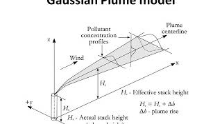
As the lecture progresses, the concept of mixing height is introduced as the intersection of environmental and adiabatic lapse rates, leading to a discussion on plume shapes and their predictability based on environmental conditions.
Further, the section dives into the fundamental transport equations involving rates of accumulation, dispersion, and flow, focusing primarily on vapor phase concentrations. The derivation of these equations includes the application of Fick's law for diffusion, emphasizing the need to model these configurations for predicting pollutant concentrations at given locations and times.
Youtube Videos


Audio Book
Dive deep into the subject with an immersive audiobook experience.
Introduction to Air Pollutant Transfer
Chapter 1 of 5
🔒 Unlock Audio Chapter
Sign up and enroll to access the full audio experience
Chapter Content
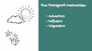
So, we were looking at box models for pollutant transfers in air. So, essentially this is a generic box model for air. The processes that we are considering in the box include advection, dispersion, reaction exchange and all that, ok.
Detailed Explanation
In this chunk, the focus is on understanding the concept of box models, which are a simplified way of representing complex environmental systems. These models help in analyzing how pollutants move through the air. By including factors like advection (movement due to wind), dispersion (spreading out of pollutants), and reactions (chemical changes), we can better understand the dynamics of air pollution.
Examples & Analogies
Imagine the box model as a fish tank where water is flowing in and out. The fish (representing pollutants) are moving around inside the tank. Advection is like the water current moving the fish along, while dispersion is the fish swimming to different parts of the tank. Reactions could be likened to fish interacting with plants or each other, affecting their health and behavior.
Understanding Atmospheric Stability
Chapter 2 of 5
🔒 Unlock Audio Chapter
Sign up and enroll to access the full audio experience
Chapter Content
So, the specific problem for air is that the height is not very well defined, so we look at what is called a mixing height and mixing height depends on a concept called stability and stability is a function of temperature in the lower atmosphere.
Detailed Explanation
Here, the concept of mixing height is introduced, which is the height where the atmosphere mixes air (and thus pollutants). The mixing height is influenced by stability, which refers to how warm or cool the air is at different heights. When temperatures decrease with height, it can lead to stable conditions, preventing pollutants from rising high in the atmosphere.
Examples & Analogies
Think of a warm soup pot. The heat causes the soup to rise and mix, creating a more stable environment. However, if you take a lid and trap steam, it creates a cooler layer above the soup. This is similar to stable atmospheric conditions where hot air can't rise freely, trapping pollution close to the ground.
Adiabatic Lapse Rate
Chapter 3 of 5
🔒 Unlock Audio Chapter
Sign up and enroll to access the full audio experience
Chapter Content
The lapse rate represented by Gamma, the adiabatic lapse rate is given as -0.0098 centigrade per kilo per meter or 9.8 centigrade per kilometer this is the adiabatic lapse rate. This is the dry adiabatic lapse rate.
Detailed Explanation
The adiabatic lapse rate is a critical concept in meteorology and atmospheric sciences. It describes how the temperature of a rising air parcel changes as it ascends through the atmosphere. Specifically, it states that for every kilometer up you go, the temperature drops by about 9.8 degrees Celsius. This is important because it helps predict how pollutants will behave as they move upward in the atmosphere.
Examples & Analogies
Consider climbing a mountain. As you hike higher, you often feel colder; this is because the air temperature decreases with altitude. Similarly, when pollutants are released into the air, they cool down as they rise, which can impact their dispersion and potential effects on air quality.
Potential Temperature
Chapter 4 of 5
🔒 Unlock Audio Chapter
Sign up and enroll to access the full audio experience
Chapter Content
There is another term called potential temperature defined like this theta equals T0. This is the temperature corrected to a particular pressure, so the pressure with reference to sea level pressure.
Detailed Explanation
Potential temperature is an important concept that accounts for changes in pressure as air parcels move through the atmosphere. It helps provide a standardized temperature measure that can be compared regardless of elevation. For example, if an air parcel's temperature is measured at one pressure and needs to be evaluated at another, potential temperature helps make that conversion.
Examples & Analogies
Imagine you have a balloon filled with air at sea level; if you take that balloon to the top of a mountain, the air pressure inside the balloon changes, but the air temperature inside also adjusts based on the pressure difference. The potential temperature gives us a way to understand how that air would behave if it were at sea level pressure.
Mixing Height and Plume Behavior
Chapter 5 of 5
🔒 Unlock Audio Chapter
Sign up and enroll to access the full audio experience
Chapter Content
And we also looked at this concept of mixing height, mean mixing height as the place where the intersection of the environmental lapse rate and adiabatic lapse rate happens.
Detailed Explanation
Mixing height is where the environmental lapse rate (actual temperature change in the atmosphere) equals the adiabatic lapse rate (temperature change in a rising air parcel). This intersection is crucial because it represents the maximum height pollutants can effectively mix and rise in the atmosphere. Below this height, pollutants are more likely to concentrate, while above this height, they may disperse more effectively.
Examples & Analogies
Think of a performance stage. If you have a ceiling at a certain height (the mixing height), no matter how excited the audience (pollutants) gets, they can't rise above the ceiling. This limit affects how effectively the audience can enjoy the performance, similar to how mixing height influences pollutant behavior.
Key Concepts
-
Mixing Height: The atmospheric height where air pollutants mix with surrounding atmosphere for dispersion.
-
Atmospheric Stability: Refers to how air parcels behave in relation to temperature changes as they rise or sink in the atmosphere.
-
Adiabatic Lapse Rate: The temperature decrease of an air parcel as it ascends without heat exchange.
-
Potential Temperature: A normalized temperature measurement of an air parcel with respect to pressure changes.
-
Fick's Law: A foundational principle that explains the diffusion of substances in terms of concentration gradients.
Examples & Applications
An example of mixing height is the boundary layer in the atmosphere where pollutants from urban areas mix with clean air.
When modeling air quality in a city, potential temperature helps meteorologists understand temperature inversions and pollution trapping.
Memory Aids
Interactive tools to help you remember key concepts
Rhymes
When air goes up, it cools down, that's the rate called lapse all around.
Stories
Imagine a balloon (the air parcel) rising high, as it ascends, it cools and makes the wispy clouds in the sky.
Memory Tools
SHEAR = Stability, Height, Environmental lapse rate, Adiabatic lapse, and Reaction is a guide for atmospheric layers.
Acronyms
P.E.A.C.E. for Potential temperature
Pressure-corrected temperature
Environmental stability
Adiabatic lapse
and Concentration equalization.
Flash Cards
Glossary
- Mixing Height
The height in the atmosphere where maximum mixing of pollutants occurs.
- Atmospheric Stability
The behavior of an air parcel in the atmosphere concerning its ascent or descent.
- Adiabatic Lapse Rate
The rate at which air temperature decreases with an increase in altitude, approximated as -0.0098 °C/m.
- Potential Temperature
The temperature of an air parcel, corrected for pressure changes, allowing for comparison across altitudes.
- Fick's Law
A principle that describes diffusion; states that the flux of a substance is proportional to its concentration gradient.
Reference links
Supplementary resources to enhance your learning experience.