
Fick’s Law and Its Application
Enroll to start learning
You’ve not yet enrolled in this course. Please enroll for free to listen to audio lessons, classroom podcasts and take practice test.
Interactive Audio Lesson
Listen to a student-teacher conversation explaining the topic in a relatable way.
Understanding Atmospheric Stability
🔒 Unlock Audio Lesson
Sign up and enroll to listen to this audio lesson

Today, we will understand how atmospheric stability affects the dispersion of air pollutants. Can anyone tell me what atmospheric stability means?

Is it how stable the air conditions are in the environment?
Exactly! Atmospheric stability refers to how an air parcel behaves as it rises. A stable atmosphere limits vertical movement, making it difficult for pollutants to disperse.

How do temperature gradients relate to this?
Great question! The environmental lapse rate is critical. It tells us how temperature changes with height and influences stability. A negative lapse rate indicates rising air is warmer than its surroundings, promoting dispersion!

So, if the lapse rate is constant, does that mean the stability won't change?
Yes, the adiabatic lapse rate remains constant. Remember: stability affects how pollutants are managed in the atmosphere!
To summarize, stability affects pollutant behavior based on temperature gradients. Make sure to keep this in mind!
Fick’s Law Overview
🔒 Unlock Audio Lesson
Sign up and enroll to listen to this audio lesson

Let’s talk about Fick’s Law and its role in diffusion. Who can give me a brief explanation of what diffusion means?

Isn’t diffusion the process where particles spread from an area of high concentration to low concentration?
Correct! Fick's Law helps us quantify this process mathematically. It relates the diffusion flux to the concentration gradient.
What does flux mean in this context?
Flux is the amount of substance passing through a unit area per unit time. According to Fick's First Law, it's proportional to the concentration gradient.
Could you help us visualize how this works in air pollution?
Certainly! Imagine a factory emitting pollutants. Fick's Law describes how that concentration diminishes as you move away from the source.
In summary, Fick’s Law is crucial in environmental engineering as it helps assess and predict pollutant dispersion, which is vital for air quality management.
Mixing Height and Plume Formation
🔒 Unlock Audio Lesson
Sign up and enroll to listen to this audio lesson
Next, let's discuss mixing height and how it relates to pollutant dispersion. Can anyone explain what mixing height refers to?
Is it the height where different air layers mix?
Exactly! The mixing height represents the layer where environmental laps rate matches the adiabatic lapse rate, impacting how pollutants are dispersed in the atmosphere.
What’s the significance of understanding this height?
Understanding mixing height helps predict the extent of pollutant vertical spread. It directly influences air quality assessments.
Can you give us an example?
Certainly! If pollutants are released below mixing height, they may not disperse effectively, leading to higher local concentrations. This is crucial for health assessments!
To summarize, mixing height is key in understanding vertical dispersion of pollutants, directly affecting environmental quality.
Introduction & Overview
Read summaries of the section's main ideas at different levels of detail.
Quick Overview
Standard
In this section, we explore Fick’s Law, its role in predicting pollutant concentration in air, and the concept of mixing height driven by atmospheric stability. The section details how the environmental lapse rate influences air parcels and the application of Fick’s Law in modeling pollutant transport.
Detailed
Fick’s Law and Its Application
Fick's Law is foundational in understanding how substances diffuse, particularly in environmental contexts such as air quality control. In this section, we first introduce the concept of mixing height, which describes the vertical extent of air mixing influenced by atmospheric stability. Stability is determined by factors like temperature gradients (the environmental lapse rate).
We note how an air parcel's behavior during adiabatic processes dictates its movement, and we calculate the adiabatic lapse rate (-0.0098 °C/m) derived from thermodynamic relations. This knowledge is critical for environmental modeling as it informs the behavior of pollutants released into the air. The concept of potential temperature is also introduced, helping normalize temperature measurements for varying pressures.
A significant concept discussed is the 'plume,' which describes the shape and behavior of pollutant dispersion as it rises through the atmosphere. By utilizing Fick’s Law, we derive the necessary equations to model the transport of pollutants within a defined volume, detailing how factors like wind and dispersion contribute to concentration levels at certain distances from the source.
Overall, this section is pivotal for students in chemical engineering and environmental studies, providing them with the necessary tools to analyze and predict air quality conditions.
Youtube Videos


Audio Book
Dive deep into the subject with an immersive audiobook experience.
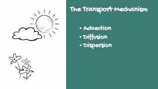
Overview of the Transport Model
Chapter 1 of 4
🔒 Unlock Audio Chapter
Sign up and enroll to access the full audio experience
Chapter Content
Our goal is to predict concentration as a function of place and time (x, y, z, and time). We consider one control volume within the plume, where the pollutant is moving.
Detailed Explanation
This chunk introduces the main objective of the transport model we are studying: to predict the concentration of pollutants in a given area over time. By modeling a specific volume of air where pollutants might exist, we focus on how these pollutants are distributed and transported. The coordinates (x, y, z) help us define the location in three-dimensional space, which, combined with time, provides a comprehensive view of pollutant movement.
Examples & Analogies
Imagine you're in a room where someone is spraying a perfume. Over time, the scent spreads throughout the room. By observing the strength of the scent at different locations (like the corners of the room), we can understand how quickly and in what pattern the perfume disperses. This is similar to how we analyze pollutant concentrations in the air.
Understanding Flux and Accumulation Rates
Chapter 2 of 4
🔒 Unlock Audio Chapter
Sign up and enroll to access the full audio experience
Chapter Content
We model the box with dimensions delta x, delta y, and delta z, identifying processes such as accumulation, flow in, flow out, dispersion, and reactions.
Detailed Explanation
Here, we are breaking down how we mathematically model the movement and concentration of pollutants. The dimensions of the box (delta x, delta y, delta z) represent the volume we're studying. The term 'accumulation' refers to how much pollutant builds up in this volume versus how much flows in or out and how it spreads due to dispersion. By understanding these processes, we can create an equation that describes how pollutants behave in the environment.
Examples & Analogies
Consider a bathtub filled with water. If you pour water in (flow in) but also have a drain (flow out), the water level (representing concentration) will change depending on how fast you're pouring versus how fast the drain is working. This balance helps us understand how pollutants 'accumulate' in our defined control volume.
Application of Fick's Law
Chapter 3 of 4
🔒 Unlock Audio Chapter
Sign up and enroll to access the full audio experience
Chapter Content
The equation for flux, described by Fick’s law, is represented as a negative gradient indicating that pollution tends to move from high to low concentrations.
Detailed Explanation
In this context, we apply Fick's law to describe how pollution disperses. The law states that the flux (the rate of flow of pollutants) is proportional to the concentration gradient. When there's a higher concentration of pollutants in one area, they tend to move towards areas with lower concentrations, which is depicted in the equation as a negative sign. This is fundamental because it helps us predict how pollutants will spread through the air.
Examples & Analogies
Think of a dropped food coloring in water. If you drop it in a corner of a clear glass, the color will spread throughout the water over time, moving from the area of high concentration (where you dropped it) to areas of lower concentration (clear water). Fick’s Law describes this natural tendency of materials to spread out evenly.
Formulating the Transport Model
Chapter 4 of 4
🔒 Unlock Audio Chapter
Sign up and enroll to access the full audio experience
Chapter Content
We construct our equations by considering the rate of dispersion, with the flow in one direction only. The resulting equation summarizes all the contributing factors.
Detailed Explanation
In this section, we discuss how to write mathematical equations that embody our model of pollutant transport. We assume that pollutants primarily flow in the x-direction and express the changes in concentration over time due to dispersion. The resulting equations help us quantify the impacts of different parameters on pollutant concentration, allowing for predictions about how pollutants will behave under various conditions.
Examples & Analogies
Returning to our bathtub analogy, if we focus only on the water pouring in from one faucet and the drain only on one side, we can create a simple equation to describe the water level's changes. In pollution modeling, we simplify complex real-world inputs to make useful predictions about how pollutants disperse.
Key Concepts
-
Atmospheric Stability: It influences the vertical movement of air and pollutant dispersion.
-
Fick’s Law: A fundamental principle describing how substances distribute in space over time.
-
Mixing Height: The layer in the atmosphere where pollutants are effectively mixed and dispersed.
Examples & Applications
When a factory emits smoke, the mixing height determines how far that smoke can rise before dispersing into the atmosphere.
In stable atmospheric conditions, pollutants may remain concentrated near the ground instead of dispersing.
Memory Aids
Interactive tools to help you remember key concepts
Rhymes
When air is stable, pollution stays low; let the lapse rates guide how they flow.
Stories
Imagine a hot air balloon rising slowly. If the air around it is warmer, it floats high; but in colder air, it sinks, much like pollutants are trapped near the ground when atmospheric stability is high.
Memory Tools
Remember 'MAP' for Mixing height, Adiabatic lapse rate, and Pressure norms to understand air behavior.
Acronyms
FICK - Flux, Input, Concentration, Kinetics. It’s all about how particles are moving!
Flash Cards
Glossary
- Atmospheric Stability
The tendency of the atmosphere to resist vertical motion, affecting pollutant dispersion.
- Environmental Lapse Rate
The rate at which the temperature of the atmosphere decreases with an increase in altitude.
- Adiabatic Lapse Rate
The rate of temperature change of an air parcel as it rises without exchange of heat.
- Mixing Height
The height at which the environmental lapse rate intersects the adiabatic lapse rate, influencing pollutant dispersion.
- Fick’s Law
A principle that describes diffusion, relating flux to concentration gradient.
- Flux
The amount of substance that passes through a unit area in a unit of time.
- Plume
The cloud of air pollutants released into the atmosphere and its shape while dispersing.
Reference links
Supplementary resources to enhance your learning experience.