
Generalized Transport Model
Enroll to start learning
You’ve not yet enrolled in this course. Please enroll for free to listen to audio lessons, classroom podcasts and take practice test.
Interactive Audio Lesson
Listen to a student-teacher conversation explaining the topic in a relatable way.
Introduction to Pollutant Transport
🔒 Unlock Audio Lesson
Sign up and enroll to listen to this audio lesson

Today we'll explore how pollutants are transferred in the air using a generalized transport model. Can anyone tell me what we mean by 'pollutant transport'?

Is it how pollutants spread from one place to another?
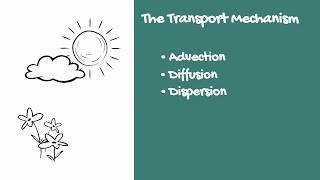
Exactly! Pollutant transport involves advection, dispersion, and other processes that affect how pollutants are distributed. Remember, the key processes can be summarized with the acronym A.D.R. Can anyone expand on what those processes entail?

Advection is the movement with wind, right?
Correct! And dispersion refers to the spreading out of pollutants due to turbulence. Very good.

What about reaction? How does that fit in?
Great question! Reactions can change the chemical composition of pollutants as they move, adding complexity to our models. Let's continue exploring these concepts.
Mixing Height and Atmospheric Stability
🔒 Unlock Audio Lesson
Sign up and enroll to listen to this audio lesson

Now, let’s focus on mixing height. Can anyone tell me what affects the mixing height in the atmosphere?

Is it related to temperature?
Very insightful! Yes, the mixing height is influenced by atmospheric stability, which varies with temperature gradients. Who can define atmospheric stability?
It's how a parcel of air behaves when it moves up or down in the atmosphere.
Excellent explanation! Stability affects how pollutants are mixed and transported vertically.
What about the lapse rate? How does that play in?
The lapse rate helps define the environmental temperature gradient and is crucial in determining mixing height.
The Generalized Transport Model Equation
🔒 Unlock Audio Lesson
Sign up and enroll to listen to this audio lesson
Next, let's get into the mathematical aspect. Who remembers the basic structure of the transport model equation?
Is it about the rate of accumulation relating to the rates of flow in and out?
Correct! The equation balances accumulation with flow and dispersion. Can anyone mention the role of Fick's Law in this context?
It relates the flux to concentration gradients, right?
Exactly! This law gives us a fundamental understanding of how substances diffuse through the air. Let’s practice writing these equations together.
Practical Applications and Implications
🔒 Unlock Audio Lesson
Sign up and enroll to listen to this audio lesson
Now, how can we apply our model in real scenarios? Why is it important to predict pollutant concentration at specific locations?
It helps us understand exposure levels for people in different areas.
Exactly, and by knowing potential concentrations, we can implement control strategies! What factors could affect these predictions?
Weather conditions like wind and temperature could change how pollutants behave.
Correct! These real-world implications are crucial for environmental engineering and public health.
Introduction & Overview
Read summaries of the section's main ideas at different levels of detail.
Quick Overview
Standard
The section explains the complexities of modeling air pollution, focusing on concepts such as mixing height, atmospheric stability, and the generalized transport model equations encompassing various processes impacting pollutant transport.
Detailed
In this section, we delve into the generalized transport model as applied to pollutant transfers in the air, particularly focusing on how air mixes and how pollutants disperse within this medium. The discussion begins by introducing the concept of the mixing height, which varies based on atmospheric stability — a condition influenced by temperature gradients in the lower atmosphere. The lapse rate, representing how temperature changes with altitude, is critical in understanding these dynamics. The section covers the definition of potential temperature and its role in modeling, emphasizing the need for a clear understanding of environmental parameters. The generalized transport model incorporates processes like advection, dispersion, and reaction to provide a comprehensive framework for analyzing pollutant concentration as a function of space and time. Critical equations governing this transport are highlighted, including those derived from Fick's Law relating flux to concentration gradients. Insights into how to write these equations for different dimensions are provided, enabling students to appreciate the multifaceted nature of environmental quality modeling.
Youtube Videos


Audio Book
Dive deep into the subject with an immersive audiobook experience.
Introduction to the Generalized Transport Model
Chapter 1 of 5
🔒 Unlock Audio Chapter
Sign up and enroll to access the full audio experience
Chapter Content
Solastimewhenwewerelookingatwewerelookingatthepollutanttransport,ourgoalistobeabletopredictconcentrationasfunctionofplaceandtimex,y,zandtime.So,welookatonecontrolvolumewithintheplume,itiswherethepollutantismovingandwetrytomodelit.
Detailed Explanation
In this chunk, we discuss the purpose and framework of the generalized transport model in the context of pollutant transport. The model aims to predict how pollutants spread in the environment, specifically in air. By analyzing different control volumes, which are small sections of air, we can understand how pollutants behave over time and space. The focus on concentration as a function of coordinates (x, y, z) and time emphasizes the dynamic nature of pollution dispersion.
Examples & Analogies
Imagine trying to understand how a drop of ink disperses in a bowl of water. The ink starts from a specific point, and as time passes, it spreads out in different directions—this is similar to how pollutants disperse in the atmosphere. The control volume we study is akin to observing just a small portion of that bowl to predict how the ink will dilute and spread.
Understanding the Processes in the Model
Chapter 2 of 5
🔒 Unlock Audio Chapter
Sign up and enroll to access the full audio experience
Chapter Content
So, we did this last class, we will go over this one again. So, if you take this box which has dimensions of delta x, delta y, delta z, we have this term here rate of accumulation equals rate of in by flow or rate out by flow, rate in by dispersion, rate out by dispersion.
Detailed Explanation
This chunk explains the fundamental balance of the transport model, focusing on the concepts of flow and dispersion. In a defined control volume with specific dimensions (delta x, delta y, delta z), we analyze how pollutants accumulate. The 'rate of accumulation' is determined by the rate of pollutants entering the box (flow) and the rate leaving, along with dispersion, which refers to how pollutants spread within that volume. Essentially, it forms the basis of how we model changes in pollutant concentration.
Examples & Analogies
Think of filling a bathtub with water. The rate at which the water is being added is similar to the rate of flow coming into the control volume, while the rate at which it drains represents the outflow. If you also consider how the water mixes and spreads throughout the tub, you can relate this to dispersion, showing how pollutants distribute themselves in a given area.
Components of the Generalized Transport Model
Chapter 3 of 5
🔒 Unlock Audio Chapter
Sign up and enroll to access the full audio experience
Chapter Content
The transport model can have anything the generalized transport model will also have a reaction, will also have adsorption, will also have deposition all these things will happen this multi-phase model but we are not doing that here we are looking at only.
Detailed Explanation
In this chunk, the various processes incorporated into the generalized transport model are highlighted. While the model can account for several factors (such as reactions, adsorption, and deposition), the current focus is on a specific component, emphasizing the vapour phase concentration. This simplification allows for a clearer understanding of pollutant dynamics without delving into the complexities of multi-phase interactions at this stage.
Examples & Analogies
Consider cooking a dish that requires several ingredients. At times, you may only focus on one key ingredient to understand its flavor before combining it with others later. Here, understanding the vapour phase concentration serves as that initial ingredient that helps build our understanding of pollutant transport before considering all the other reactions and interactions.
Determining Exposure Concentration
Chapter 4 of 5
🔒 Unlock Audio Chapter
Sign up and enroll to access the full audio experience
Chapter Content
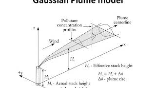
What we are interested in this case is that say, I am interested in this person standing here on the ground and what is the concentration that you are being exposed to, ok, so from this point of view I would like to know if this plume is going to travel to this person standing at a distance of 5 kilometers or some place.
Detailed Explanation
In this chunk, we focus on the relevance of the model in predicting pollutant concentration to individuals in specific locations, such as a person standing on the ground. Understanding how a plume – the visible stream of smoke or pollutants – moves and whether it will reach people at various distances is crucial for assessing exposure risks. It highlights the practicality of the model in real-life situations where human health and safety may be at stake.
Examples & Analogies
Imagine a fireworks display, where you want to know if the smoke will reach a crowd gathered at a safe distance. By modeling the smoke's trajectory and spread, you can predict whether attendees will be affected, just as we use models to determine if pollutants will impact people living in the surrounding areas of a pollution source.
The Role of Dispersion in the Model
Chapter 5 of 5
🔒 Unlock Audio Chapter
Sign up and enroll to access the full audio experience
Chapter Content
So, in this equation, we write this rate of dispersion. This flux term, this is flux multiplied by area.
Detailed Explanation
This chunk introduces the concept of dispersion within the model, specifically focusing on how flux relates to area. Dispersion signifies the process by which pollutants spread out. The equation involves calculating how much pollutant moves through a given area, providing insight into how pollutants disperse in the environment. Understanding this relationship is critical for accurately modeling pollutant transport.
Examples & Analogies
Think of pouring syrup over ice cream. The syrup spreads over the surface area of the ice, and you can control how thick the syrup layer is by adjusting the pouring area. In the same way, dispersion models help us understand how pollutants spread over an area, helping us gauge their impact as they move and dilute in the atmosphere.
Key Concepts
-
Generalized Transport Model: A framework for analyzing pollutant transport in the air incorporating advection, dispersion, and reactions.
-
Mixing Height: The altitude at which effective turbulence and mixing occur, significantly influenced by atmospheric stability.
-
Atmospheric Stability: Determines how pollutants will disperse vertically in the atmosphere based on thermal gradients.
Examples & Applications
Example 1: If a factory emits pollutants at a height above the mixing layer, those pollutants may not disperse effectively, leading to higher concentrations near the ground.
Example 2: During a stable atmospheric condition at night, pollutants may become trapped at lower altitudes, increasing local pollution levels.
Memory Aids
Interactive tools to help you remember key concepts
Rhymes
Pollutants ride the windy tide, advection carries them wide, mixing height up high, where the skies comply.
Stories
In a bustling valley, a factory puffed smoke as the sun set. The cool air trapped the smoke low, revealing the tale of atmospheric stability's role in pollutant spread.
Memory Tools
A.D.R. for pollutant transport — Advection, Dispersion, Reaction.
Acronyms
S.T.A.M. for stability factors
Sunlight
Temperature
Air Pressure
Mixing processes.
Flash Cards
Glossary
- Advection
The transport of substances by the bulk motion of the fluid, commonly attributed to wind in atmospheric contexts.
- Dispersion
The spreading of pollutants within the air due to turbulence and mixing mechanisms.
- Mixing Height
The height in the atmosphere above which significant mixing occurs due to turbulence.
- Atmospheric Stability
The tendency of an air parcel to resist vertical movement, influenced by temperature gradients.
- Lapse Rate
The rate at which atmospheric temperature decreases with an increase in altitude.
- Fick's Law
A principle that describes diffusion and establishes a relationship between flux and concentration gradient.
Reference links
Supplementary resources to enhance your learning experience.