
Modeling Pollutant Transport
Enroll to start learning
You’ve not yet enrolled in this course. Please enroll for free to listen to audio lessons, classroom podcasts and take practice test.
Interactive Audio Lesson
Listen to a student-teacher conversation explaining the topic in a relatable way.
Box Models and Pollutant Transport Basics
🔒 Unlock Audio Lesson
Sign up and enroll to listen to this audio lesson

Today, we are going to discuss box models of pollutant transport in the atmosphere. Can anyone explain what a box model represents?

Is it a simplified way to understand how pollutants move through air?
Exactly! Box models help us visualize processes like advection and dispersion that influence how and where pollutants travel. Can anyone tell me what advection means?

It's the movement of pollutants with the wind, right?
Yes! And dispersion is another process that's crucial. It refers to how pollutants spread out due to turbulence and other factors. Remember the acronym A&D for Advection and Dispersion!

Got it! A&D for understanding pollutant transport.
Great! Now, let’s discuss atmospheric stability since it significantly affects how pollutants behave.
Atmospheric Stability
🔒 Unlock Audio Lesson
Sign up and enroll to listen to this audio lesson

The stability of an air parcel is crucial for understanding pollutant dispersion. What do you think stability means in this context?

Is it about how warm or cold an air parcel is compared to the surrounding air?
That's correct! Stability determines if an air parcel will rise or descend. If it's warmer than its surroundings, it will rise—a process known as adiabatic expansion. Does anyone know the definition of the adiabatic lapse rate?
Isn't it about how temperature decreases with altitude, around -0.0098 °C per meter?
Exactly! That’s a key figure. Just remember the value, and you'll recognize how it affects air movement. Keep that in mind as we continue.
Potential Temperature and Mixing Height
🔒 Unlock Audio Lesson
Sign up and enroll to listen to this audio lesson
Now, let’s discuss potential temperature. Can someone explain its significance?
It corrects the temperature of an air parcel as it moves from one pressure to another.
Exactly! And it helps us understand how pollutants mix in the atmosphere. Another crucial concept is mixing height. Why do you think it's important?
It determines where pollutants can accumulate and disperse in the atmosphere.
Yes! The mixing height is the height at which the environmental lapse rate intersects the adiabatic lapse rate. If you remember the term MIxing height, think of it as the 'Mixing Interference height'.
Transport Model Application
🔒 Unlock Audio Lesson
Sign up and enroll to listen to this audio lesson
Finally, let's put this all together. How can we use the transport model to predict pollutant concentration?
We can create equations based on the rates of accumulation, inflow, and outflow of the pollutants.
Yes! These processes are captured in the equation to determine how concentration changes over time and space. Who can summarize what goes into that model?
We account for flow due to wind, dispersion effects, and reaction rates where necessary.
Perfect summary! Make sure to think about how these models can help predict real-world situations of exposure.
Introduction & Overview
Read summaries of the section's main ideas at different levels of detail.
Quick Overview
Standard
In this section, we explore how pollutants are transported in the air using box models. We cover critical concepts such as atmospheric stability, potential temperature, mixing height, and the equations governing advection and dispersion, emphasizing their implications for environmental quality and pollutant concentration prediction.
Detailed
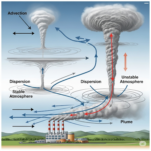
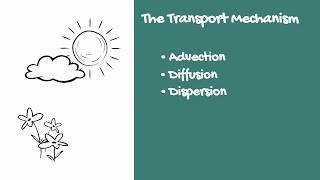
This section on Modeling Pollutant Transport delves into the complexities of how pollutants are transferred in the atmosphere, primarily through the lens of box models that represent air pollution dynamics. Key processes under consideration include advection, which describes the movement of pollutants with air flow, and dispersion, which refers to the spreading of pollutants due to turbulence and other factors.
One essential concept discussed is atmospheric stability, which influences how pollutants ascend and disperse into the air. The stability of air parcels refers to how they behave when they rise in the atmosphere, influenced by the adiabatic lapse rate, defined as the temperature change of the air with elevation (approximately -0.0098 °C per meter). The concepts of potential temperature and mixing height are also examined, illustrating how temperature corrections and environmental gradients define the regions where pollutants can accumulate or disperse.
Furthermore, the section introduces a generalized transport model to analyze the flow of gas in the atmosphere, touching on critical factors such as reaction and deposition. Awareness of pollutant exposure at specific locations is highlighted, bringing into focus how these modeling techniques can predict the concentration of pollutants that individuals may encounter in real-world scenarios. The session urges students to understand these dynamics deeply, stressing that a solid grasp of these basic principles can aid in complex modeling tasks related to environmental science.
Youtube Videos


Audio Book
Dive deep into the subject with an immersive audiobook experience.
Introduction to Pollutant Transport
Chapter 1 of 5
🔒 Unlock Audio Chapter
Sign up and enroll to access the full audio experience
Chapter Content
So, last time when we were looking at the pollutant transport, our goal is to be able to predict concentration as function of place and time x, y, z and time. So, we look at one control volume within the plume, it is where the pollutant is moving and we try to model it.
Detailed Explanation
In this introduction, the key concept is to understand that pollutant transport refers to predicting how much of a pollutant is present in different locations (x, y, z) over time. Scientists create a 'control volume,' which is a specific area in the environment where they can observe and measure the movement of pollutants. The model helps in estimating how pollutants disperse in the air.
Examples & Analogies
Imagine you're watching smoke rising from a campfire. To understand how the smoke spreads through the air, you might look at a specific area around the campfire—the volume of air where the smoke is likely to be. Similarly, when scientists study air pollution, they focus on certain volumes of air to determine how pollutants travel and change over time.
Fundamentals of the Transport Model
Chapter 2 of 5
🔒 Unlock Audio Chapter
Sign up and enroll to access the full audio experience
Chapter Content
So, if you take this box which has dimensions of delta x, delta y, delta z, we have this term here rate of accumulation equals rate of in by flow or rate out by flow, rate in by dispersion, rate out by dispersion.
Detailed Explanation
In modeling pollutant transport, scientists conceptualize the environment as a box (or control volume) with specific dimensions (delta x, delta y, delta z). They use mathematical relationships to describe how pollutants enter and leave this box. The 'rate of accumulation' refers to the change in pollutant concentration within this box. It is influenced by different factors: flow (how much pollutant enters or exits due to wind), and dispersion (how pollutants spread out in the air due to various factors like temperature changes).
Examples & Analogies
Think of a bathtub filled with water (the control volume). If you pour soap into one side of the tub (rate in by flow) and the soap spreads throughout the water (dispersion), you can measure how much soap is present at any point in the tub over time. The same principles apply to understanding how pollutants spread in the air.
Processes Influencing Pollutant Transport
Chapter 3 of 5
🔒 Unlock Audio Chapter
Sign up and enroll to access the full audio experience
Chapter Content
The transport model can have anything. The generalized transport model will also have a reaction, will also have adsorption, will also have deposition all these things will happen this multi-phase model but we are not doing that here we are looking at only A, so A is vapor phase concentration only.
Detailed Explanation
The transport model can be complex and take into account various processes that influence how pollutants behave in the atmosphere. These processes can include reactions (where pollutants change chemical forms), adsorption (where pollutants attach to surfaces), and deposition (where they settle out of the air). However, in this particular discussion, the focus is solely on the concentration of pollutants in the vapor phase (the gaseous state), simplifying the model to understand basic transport dynamics.
Examples & Analogies
Consider cooking in a kitchen with spices in the air. As you cook, the aroma (vapor) spreads throughout the kitchen (transport). If someone walks into the kitchen, they can smell the spices (concentration) due to their movement in the air. The processes affecting how the smell behaves might include sticking to kitchen surfaces (adsorption) or settling on the floor (deposition), but at the moment, we’re just focusing on how it circulates in the air.
Calculating Concentration Exposure
Chapter 4 of 5
🔒 Unlock Audio Chapter
Sign up and enroll to access the full audio experience
Chapter Content
So, what we are interested in this case is that say, I am interested in this person standing here on the ground and what is the concentration that you are being exposed to.
Detailed Explanation
In studying pollutant transport, one primary objective is to determine the concentration of pollutants that individuals are exposed to at specific locations. This is critical for understanding health risks and environmental impacts. By making calculations based on the transport model, scientists can predict how pollutants from a source (like a factory) might affect a person standing at a certain distance away.
Examples & Analogies
Imagine a smoker standing outside a café. The concentration of smoke that a person at the entrance of the café would breathe in is similar to how scientists measure pollutant levels. By analyzing wind direction and the amount of smoke, they can estimate how much the person is exposed to, just as they would with air pollution from a nearby factory.
Understanding Dispersion in Pollutant Transport
Chapter 5 of 5
🔒 Unlock Audio Chapter
Sign up and enroll to access the full audio experience
Chapter Content
So, in this equation, we write this rate of dispersion. This is a flux term, this is flux multiplied by area.
Detailed Explanation
In pollutant transport modeling, dispersion refers to the spreading of pollutants. The 'rate of dispersion' is described mathematically as the product of 'flux' (which represents the movement of pollutants through a surface) and the 'area' through which they are moving. Understanding this helps scientists predict how quickly and widely pollutants will spread in the atmosphere.
Examples & Analogies
Think of a garden hose spraying water over a flowerbed. The flow of water through the hose (flux) combined with the area it covers determines how wet the flowers get. Similarly, when scientists understand how air flows and spreads pollutants, they can estimate concentrations of harmful substances in the environment.
Key Concepts
-
Advection: Movement of pollutants with wind.
-
Dispersion: Spreading of pollutants through turbulence.
-
Atmospheric Stability: How rising or falling air behaves.
-
Adiabatic Lapse Rate: Temperature decrease with altitude.
-
Potential Temperature: Corrected temperature for pressure.
-
Mixing Height: Height defining pollutant dispersion.
Examples & Applications
In urban environments, vehicle emissions can disperse into the atmosphere, leading to varying pollutant concentrations depending on wind patterns.
During temperature inversions, stable layers of air can trap pollutants near the ground, leading to heightened pollution levels.
Memory Aids
Interactive tools to help you remember key concepts
Rhymes
Pollutants rise high, air meets its fate, the mixing height is where they accommodate.
Stories
Imagine a balloon filled with hot air rising through cooler air. As it goes up, it changes temperature, reflecting how an air parcel behaves in the atmosphere, impacting how pollutants disperse.
Memory Tools
Remember A&D for Advection and Dispersion, the two key processes in air pollution dynamics.
Acronyms
SMA (Stability, Mixing height, Adiabatic lapse) to recall vital concepts in atmospheric modeling.
Flash Cards
Glossary
- Advection
The transfer of pollutants with the wind, carrying them horizontally in the atmosphere.
- Dispersion
The process by which pollutants spread out due to turbulence and environmental factors.
- Atmospheric Stability
The tendency of an air parcel to rise or descend based on temperature differences with the surrounding air.
- Adiabatic Lapse Rate
The rate at which temperature decreases with an increase in altitude; approximately -0.0098 °C per meter.
- Potential Temperature
The temperature of an air parcel corrected for pressure changes.
- Mixing Height
The height at which the environmental lapse rate equals the adiabatic lapse rate.
Reference links
Supplementary resources to enhance your learning experience.