
Control Volume Level Equations
Enroll to start learning
You’ve not yet enrolled in this course. Please enroll for free to listen to audio lessons, classroom podcasts and take practice test.
Interactive Audio Lesson
Listen to a student-teacher conversation explaining the topic in a relatable way.
Introduction to Control Volume
🔒 Unlock Audio Lesson
Sign up and enroll to listen to this audio lesson

Good morning, class! Today we are diving into the concept of control volumes in fluid mechanics. Can anyone tell me what a control volume is?

Isn't it a specific space where we analyze fluid flow?
Exactly! A control volume is an arbitrary volume in space where we observe fluid behavior. It helps us analyze mass and energy interactions. Remember, there are different types of control volumes. Can anyone name them?

Fixed, moving, and deformable control volumes!
Great! Fixed volumes stay in one place, moving volumes travel with the fluid, and deformable ones change shape. Next, let's look at how we derive the mass conservation equation using these ideas.
Types of Control Volumes
🔒 Unlock Audio Lesson
Sign up and enroll to listen to this audio lesson

Let’s discuss each type of control volume in detail. What do you think is the significance of a fixed control volume?

It allows us to analyze flow without worrying about changes in position.
Correct! What about moving control volumes?

They adapt to fluid motion, like studying how water flows around a moving boat.
Exactly! And deformable control volumes change shape, which is important in many engineering applications. When we understand these differences, we can apply the right mass conservation equations effectively.
Mass Conservation Equation
🔒 Unlock Audio Lesson
Sign up and enroll to listen to this audio lesson
Now, let's derive the mass conservation equation. Can someone explain the Reynolds Transport Theorem?
It relates changes in a system versus changes in a control volume.
Exactly! By using it, we can express how mass flows in and out of a control volume. When we set up our mass flux equations, what variables will we consider?
Density, area, and velocity.
Correct! These basic variables will help us calculate mass flux through surfaces. Let's consider the scenario of flow through a pipe as an example.
Applications of Control Volume Analysis
🔒 Unlock Audio Lesson
Sign up and enroll to listen to this audio lesson
To conclude, let's consider real-world applications. Can anyone think of a situation where control volume analysis is crucial?
The Mars Orbiter Mission shows how fluid dynamics is vital for space travel!
Exactly! Fluid dynamics is essential to designing trajectories for spacecraft. The ability to apply conservation laws allows engineers to predict behaviors in complex systems. Remember this: control volume analysis can solve many practical problems.
Introduction & Overview
Read summaries of the section's main ideas at different levels of detail.
Quick Overview
Standard
The section elaborates on control volumes as a pivotal concept in fluid dynamics, illustrating the foundational principles of mass conservation. It outlines different types of control volumes, such as fixed, moving, and deformable, and provides insights into deriving mass conservation equations using Reynolds transport theorem.
Detailed
Detailed Summary
This section focuses on the foundational aspect of fluid mechanics, emphasizing control volume and mass conservation equations. The concept of control volume is crucial for analyzing fluid motion in various applications, as it helps to establish the flow relationship over a designated area. The section introduces different types of control volumes, including:
- Fixed Control Volume: Remains stationary in relation to a specific space.
- Moving Control Volume: Involves movement, akin to a ship navigating water.
- Deformable Control Volume: The shape of the control volume changes with time.
The section discusses how mass flows through these control volumes, leading to the mass conservation equation derived from the Reynolds transport theorem. The implications of steady and unsteady flows, along with simplifications for deriving equations, are considered, allowing for an understanding of mass influx and outflux calculations as they relate to changes in a fluid's density. Additionally, practical applications such as those seen in the Mars Orbiter Mission exemplify the theory in action, demonstrating real-world implications of fluid dynamics principles.
Youtube Videos


Audio Book
Dive deep into the subject with an immersive audiobook experience.
Introduction to Control Volume Level Equations
Chapter 1 of 8
🔒 Unlock Audio Chapter
Sign up and enroll to access the full audio experience
Chapter Content
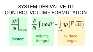
Coming back to the Reynolds transport theorems, as I derived in the last class, one is the system level equations and the other is the control volume level equations.
Detailed Explanation
In this part, we are reintroducing the concepts we learned in the previous lecture about Reynolds transport theorems. We differentiate between equations formulated at the system level and those at the control volume level. System level equations describe the behavior of a closed system, while control volume level equations allow us to analyze the flow of mass, momentum, and energy across a defined volume in space (the control volume).
Examples & Analogies
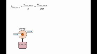
Think of a car's fuel system as a closed system (like a system level equation) where we only look at how much fuel remains in the tank without considering its movement. In contrast, if we consider the entire car (the control volume), we can analyze how fuel flows in and out as the car drives, representing a dynamic analysis of the control volume.
Understanding Extensive and Intensive Properties
Chapter 2 of 8
🔒 Unlock Audio Chapter
Sign up and enroll to access the full audio experience
Chapter Content
B: extensive property of fluid (m, ṁ, E) b: corresponding intensive property (1, ŋ, e)
Detailed Explanation
Here, we define extensive and intensive properties of fluids. Extensive properties are quantities that depend on the amount of fluid present, such as mass (m), mass flow rate (ṁ), and energy (E). Intensive properties are independent of the amount of fluid and include properties like density and specific energy. These distinctions are crucial for applying the Reynolds transport theorem since it allows us to relate these two types of properties to analyze fluid flow.
Examples & Analogies
Imagine you have a glass of water. The total amount of water (mass) is an extensive property because it changes if we add or remove water. The temperature of the water, however, is an intensive property; it doesn't change based on the glass size or how much water there is.
Mass Conservation Equation Derivation
Chapter 3 of 8
🔒 Unlock Audio Chapter
Sign up and enroll to access the full audio experience
Chapter Content
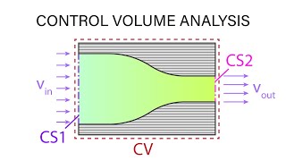
If you look at this equation, let us look it. This is the system level equations. This is what is at the control volume level. So, one talks about how this particular mass or momentum flux is crossing through the control surface.
Detailed Explanation
This chunk discusses how we derive the mass conservation equation from the Reynolds transport theorem. The equation relates how mass enters and exits a control volume through its boundaries (control surfaces). In essence, the change in mass within the control volume over time must equal the mass being transported across the surfaces of this volume, expressed mathematically as a balance between inflow and outflow.
Examples & Analogies
Consider a bathtub with a plugged drain. If you are filling it with water (inflow) and the plug is intact, the water level (mass) rises. If you pull the plug (outflow), the water will drain out. The conservation of mass states that the change in water in the tub over time equals the water being added or removed.
Steady and Unsteady Flow Analysis
Chapter 4 of 8
🔒 Unlock Audio Chapter
Sign up and enroll to access the full audio experience
Chapter Content
That means the density vary but it is steady. So, once it is steady, if you look at this term, it becomes 0. Only what remains is the surface integration part which is quite easy now.
Detailed Explanation
In fluid mechanics, flow can be categorized into steady and unsteady states. If flow is steady, properties like density do not change with time at any point in the control volume. In this case, the mathematical terms representing the time variations become zeros, simplifying the calculations. We focus on the surface integrals instead, making it easier to analyze mass flow across control surfaces.
Examples & Analogies
Think of a river flowing steadily – the water level at a specific point remains constant over time (steady flow). However, if we were to look at a rapidly changing flood situation where water heights are constantly rising or falling (unsteady flow), we'd have to account for how the water isn't static, complicating our analysis.
Applications of Control Volume Analysis
Chapter 5 of 8
🔒 Unlock Audio Chapter
Sign up and enroll to access the full audio experience
Chapter Content
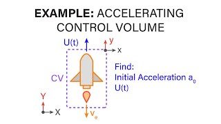
Now coming to a very interesting applications. As you know it Indian Space Research Organisation launched the satellite which is called MOM programmes...
Detailed Explanation
This section highlights the practical applications of fluid mechanics, specifically illustrating how control volume analysis is crucial in designing satellite trajectories and analyzing fluid behavior in various engineering projects. The Mars Orbiter Mission is cited as an example where understanding fluid dynamics allows engineers to calculate the correct trajectory and interactions with atmospheric forces, depending on principles derived from fluid mechanics.
Examples & Analogies
When launching a satellite, engineers calculate the rocket's path similar to how we would throw a ball across a yard – we need to know how high to throw it (angle) and how hard (momentum) to ensure it lands in the right spot (orbit around a planet). By applying control volume analysis, engineers make these critical calculations that ensure successful missions.
Relative Velocity in Moving Control Volumes
Chapter 6 of 8
🔒 Unlock Audio Chapter
Sign up and enroll to access the full audio experience
Chapter Content
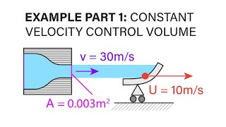
Now coming to a very interesting (()) (13:15) if I consider moving control volume like a ship which is moving with a velocity V.
Detailed Explanation
In analyzing moving control volumes, we must consider the relative velocity between the fluid flow and the moving control volume itself. By incorporating relative velocity into the equations, we can accurately describe the mass flux entering or leaving the control volume, essential for scenarios like a ship moving through water.
Examples & Analogies
Imagine a swimmer moving through water. The swimmer has their own speed, and the water is also moving (like a current). The swimmer's effective speed regarding the bank of the river differs from their speed relative to the water - this is similar to how we calculate relative velocity in moving control volumes.
Implications of Deformable Control Volumes
Chapter 7 of 8
🔒 Unlock Audio Chapter
Sign up and enroll to access the full audio experience
Chapter Content
But in case you have a deformable control volume and also moving control volume, all the things you have are complicated now.
Detailed Explanation
Deformable control volumes introduce complexity in analysis because both the fluid and control volume can change shapes and velocities with time and position. This requires careful consideration in calculations since both parameters will affect how we measure mass and momentum fluxes.
Examples & Analogies
Consider a bag filled with flour that is being squished – as you push on it, the shape changes (deforms), and so does the pressure of the flour inside. Fluid dynamics involving deformable control volumes requires understanding both how pressure and volume change under these conditions.
Summary of Conservation Principles
Chapter 8 of 8
🔒 Unlock Audio Chapter
Sign up and enroll to access the full audio experience
Chapter Content
Now, let us come to the, as I said it, we need to have three equations. One is conservation of mass, conservation of linear momentum or the angular momentum. And third is, as you know it, conservation of energy.
Detailed Explanation
In fluid mechanics, three key conservation principles guide our analyses: conservation of mass, conservation of momentum, and conservation of energy. Understanding how these principles interrelate helps engineers and scientists solve a variety of fluid flow problems effectively. While solving practical problems, often we need only two of these equations, with mass conservation being crucial.
Examples & Analogies
Think about cooking – when you bake, you have several ingredients (mass), and you must mix them (momentum) without losing anything (mass conservation). If you add heat (energy), it changes the physical properties of your mixture but, fundamentally, the quantities of each ingredient must match what you started with. Similarly, in fluid mechanics, these conservation laws ensure balance throughout any fluid system.
Key Concepts
-
Control Volume: A space where fluid flow is analyzed.
-
Fixed Control Volume: Remains in one position during the process.
-
Moving Control Volume: Changes position in coordination with fluid motion.
-
Deformable Control Volume: Shape changes over time.
-
Mass Conservation: Principle stating mass is constant in closed systems and during fluid flow.
-
Reynolds Transport Theorem: Establishes a relationship between system properties and control volume properties.
Examples & Applications
Analyzing fluid flow through a pipe using mass conservation equations.
Studying the trajectory changes of the Mars Orbiter mission, demonstrating fluid dynamics applications.
Memory Aids
Interactive tools to help you remember key concepts
Rhymes
In fluid flow, let’s take a space, / Control volumes help us find a place.
Stories
Imagine a ship sailing through the sea; the water flows around it, just like our control volume moving infinitely.
Memory Tools
Remember 'MCF' for Mass Conservation Flow: Mass stays constant for inflows and outflows.
Acronyms
CVM
Control Volume Mechanics
essential for understanding fluid motion!
Flash Cards
Glossary
- Control Volume
An arbitrary volume in space through which fluid flows, used for analysis in fluid dynamics.
- Mass Conservation Equation
An equation that describes the conservation of mass within a control volume, accounting for mass inflow and outflow.
- Reynolds Transport Theorem
A theorem that provides a relationship between the rates of change of properties in a system and control volume, essential for deriving conservation equations.
- Fluid Dynamics
The study of fluids in motion and the forces acting upon them.
- Density
The mass per unit volume of a substance, a key factor in fluid flow calculations.
Reference links
Supplementary resources to enhance your learning experience.