
Definitions of Material Derivative
Enroll to start learning
You’ve not yet enrolled in this course. Please enroll for free to listen to audio lessons, classroom podcasts and take practice test.
Interactive Audio Lesson
Listen to a student-teacher conversation explaining the topic in a relatable way.
Understanding Material Derivative
🔒 Unlock Audio Lesson
Sign up and enroll to listen to this audio lesson

Today, we will explore the concept of the material derivative in fluid dynamics. To start, can anyone tell me what a derivative typically represents in physics?

It represents the rate of change of one quantity with respect to another.
Exactly! Now, a material derivative takes that a step further. It measures how a quantity changes as it moves along with a particle in the fluid. This means we need to consider both time and space changes. Can anyone think of why that's important?

Because fluids can be moving and changing at the same time, so we need to capture both effects!
Right! Think of it this way: the velocity of a fluid particle can change due to local influences at a point, and because it is moving through different regions of varying velocity. We often classify these changes as local acceleration and convective acceleration. Can anyone summarize these concepts?

Local acceleration is the change you feel if you're at a point, and convective acceleration is what happens because the particle is moving through different velocities.
Great summary! Remember the acronym LAC: Local and Convective acceleration.
To recap, the material derivative accounts for how quantities shift with the motion of fluid particles. Let's keep these concepts in mind as we progress.
Mathematical Representation
🔒 Unlock Audio Lesson
Sign up and enroll to listen to this audio lesson

Now let's delve deeper into the mathematical representation. Who can recall the standard form of the material derivative?

Isn’t it something like the total derivative with respect to time?
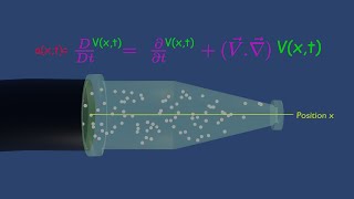
Yes! The material derivative incorporates both local and convective effects. Its general formula is given as: Dφ/Dt = ∂φ/∂t + V · ∇φ, where φ represents any field variable. Does that make sense?
Could you explain what the terms mean?
Sure! The first term is the local time derivative, which measures how φ changes at a point. The second term considers how φ changes as the particle moves through varying fields in space. This operator D reflects our focus on the particle trajectory. Can someone think of an example where this might be applied?
In weather systems! It would help us understand how temperature and pressure change as air moves.
Exactly! Understanding these changes is essential in meteorology, fluid dynamics, and engineering applications, among others. Let's ensure we grasp this formula thoroughly.
Application Examples
🔒 Unlock Audio Lesson
Sign up and enroll to listen to this audio lesson
Now let's look at how we use material derivatives in calculations. Suppose we have a velocity field V defined as V = zi + xj + yk. How would we compute the material derivative?
We would plug it into our formula, right?
Right! We need to find out the velocity components at a specific point first, then calculate the derivative. What do we get at the coordinates (1, 4, 1)?
The velocities would be u = 1, v = 4, and w = 1.
Correct! Now, substituting those values, what do we find for the acceleration components?
We would compute the partial derivatives of each component and combine them?
Exactly! Remember to check if any additional terms appear in our calculations for local versus convective acceleration. Each part sheds light on different dynamics at play. Great work, everyone!
Comparison of Frames
🔒 Unlock Audio Lesson
Sign up and enroll to listen to this audio lesson
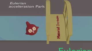
Next, let's compare the Lagrangian and Eulerian frameworks for analyzing fluid motion. Who can explain the key difference?
Lagrangian focuses on the motion of individual particles, while Eulerian looks at the fluid properties at a fixed point in space.
Great explanation! This distinction affects how we apply the material derivative—can anyone elaborate further?
In Lagrangian analysis, we track particles themselves, while in Eulerian analysis, we observe the overall flow field.
Exactly! Each perspective offers unique values in different applications. For instance, meteorologists often use the Eulerian approach, while particle tracking in simulations aligns more with the Lagrangian perspective. Why do you think these differences matter in practice?
Each method provides different insights. Depending on the application, one might represent the fluid dynamics more accurately than the other.
Precisely! Moving forward, we'll explore topics where these frameworks apply based on real-life dynamics. Keep reflecting on how these concepts interconnect.
Introduction & Overview
Read summaries of the section's main ideas at different levels of detail.
Quick Overview
Standard
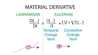
This section delves into the material derivative, focusing on its meaning as the total derivative pertaining to a fluid particle's motion through a velocity field. It contrasts Lagrangian and Eulerian perspectives and explains key concepts like local and convective acceleration, supported by mathematical expressions for fluid dynamics.
Detailed
Detailed Summary
The material derivative is a fundamental concept in fluid dynamics, describing the total change in a fluid's properties as a particle moves through space and time. Unlike standard derivatives, which provide instantaneous rates of change, the material derivative considers both temporal and spatial changes, revealing how properties such as velocity, pressure, and density evolve due to both local effects and the motion through the velocity field.
Key Concepts Addressed
- Velocity and Acceleration: The section relates Newton's second law to fluid motion, explaining that acceleration is derived as a time derivative of velocity, and emphasizing that both velocity and acceleration are vector quantities.
- Local vs. Convective Acceleration: The distinction between local acceleration (change at a fixed point) and convective acceleration (change due to motion within spatial gradients) is clarified. This duality is critical in interpreting fluid behavior.
- Material Derivative Definition: The material derivative is mathematically defined with respect to particle motion and connects both Lagrangian (particle-following) and Eulerian (field-based) perspectives.
- Applications: Examples illustrate how the material derivative helps in understanding fluid flows and can be utilized in computational problems involving velocity and acceleration fields in different coordinates.
This section lays the groundwork for further topics in fluid motion and deformation and emphasizes the role of fluid particle tracking for diverse applications in engineering and science.
Youtube Videos

![Material derivative [Fluid Mechanics #3a]](https://img.youtube.com/vi/dIGMArhv7Fc/mqdefault.jpg)
Audio Book
Dive deep into the subject with an immersive audiobook experience.
Understanding Acceleration of Fluid Particles
Chapter 1 of 5
🔒 Unlock Audio Chapter
Sign up and enroll to access the full audio experience
Chapter Content
Now, let us look at the particle levels, if I had to find out what is the acceleration of the fluid particles? Is nothing else is a time derivative of velocity of the particles, as you know it from class 10, 11th, and 12th. I am just doing this time derivative of the velocity; particle velocities with respect to time and that is what represents the accelerations, at the particles levels you will have these.
Detailed Explanation
In fluid mechanics, we define the acceleration of fluid particles as the change in their velocity over time. This concept is taught in earlier physics classes where students learn about derivatives. A derivative shows how a quantity changes with respect to another quantity—here, we are looking at how the velocity of fluid particles changes as time progresses. When we talk about particle velocity, we refer to how fast a specific fluid particle is moving at that moment. Thus, the acceleration can be mathematically represented as the derivative of velocity concerning time.
Examples & Analogies
Think of driving a car. When you press the gas pedal, the car's speed increases—this change in speed is acceleration. Similarly, in fluids, as the particles move, their speed changes over time, which we measure as acceleration.
Local and Global Components of Acceleration
Chapter 2 of 5
🔒 Unlock Audio Chapter
Sign up and enroll to access the full audio experience
Chapter Content
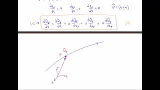
Now, if you look at this the velocities has a variability in a positions and the time because of that though when you define a; derivative with respect to time you will have a local component okay, you will have a with a x particle directions, y particle directions and z particle direction.
Detailed Explanation
When analyzing fluid flow, it’s important to recognize that the acceleration can be affected not just by time but also by the position of the particles in space, which introduces local variations. This variability is assessed by considering changes in velocities in the three spatial dimensions: x, y, and z. Therefore, when calculating derivatives, we can break them into components: local acceleration that deals with how particle velocity changes at a specific point, and multi-directional components that reflect motion in different spatial axes.
Examples & Analogies
Imagine watching a balloon being blown in the wind. The balloon's speed can change not only as time goes by (if the wind gets stronger) but also depending on where the balloon is in the gusts of wind (it may speed up or slow down based on the air currents around it).
Taylor Series and Fluid Dynamics
Chapter 3 of 5
🔒 Unlock Audio Chapter
Sign up and enroll to access the full audio experience
Chapter Content
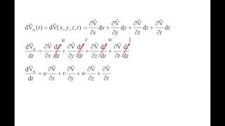
This is nothing else if you are considering is a 2 variables like I just discussed you the Taylor series, if you remember it defining for the 2 variables in this case, I have a Taylor series of 4 variables the x, y, z and the t.
Detailed Explanation
The Taylor series is a mathematical tool used to approximate functions with polynomial expressions. In fluid dynamics, we apply the Taylor series to represent the behavior of fluid particles as variables change in time and space. Specifically, by considering multiple dimensions like x, y, z, and t, we can develop a more accurate representation of how velocity and other properties behave in the fluid, allowing for deeper analysis of fluid motion.
Examples & Analogies
Think of it like trying to predict the path of a soccer ball. By using an approximate formula that accounts for its initial speed (x, y, z) and time (t), you can estimate where it will land. The more variables you add (air resistance, angle of kick, etc.), the closer your prediction will become to the real outcome.
Material Derivative Concept
Chapter 4 of 5
🔒 Unlock Audio Chapter
Sign up and enroll to access the full audio experience
Chapter Content
But many of the times people talk about the material derivative, it is nothing else, it is that the change it is a special name of material derivative means, when you talk about a particles along the particles, you compute the derivative with respect to time is a total derivative or the material derivative.
Detailed Explanation
The material derivative is a specific type of derivative that reflects how a property changes as you move with the fluid. Unlike regular derivatives that consider the change of a property solely with respect to time or space, the material derivative considers both effects simultaneously. Essentially, it allows us to track how a particle's property (like velocity, density, etc.) changes as it flows along with the fluid. This makes it particularly useful for understanding the dynamics of fluid flow.
Examples & Analogies
Imagine you are swimming in a river. The water brings along leaves and bits of debris. The properties of the water (like its temperature, speed, or even the amount of debris) change as you move downriver with it. The material derivative helps capture those changing properties as you go along with the current.
Local vs. Convective Acceleration
Chapter 5 of 5
🔒 Unlock Audio Chapter
Sign up and enroll to access the full audio experience
Chapter Content
So, if I put it that I will get the accelerations fields as I explaining it that, I will have a particle, the change of the position the particles in the x direction with respect to time will give you the velocity component in that directions, so this is for x component, so y component, z component, so the finally this accelerations will have this form.
Detailed Explanation
Acceleration within a fluid can be categorized into two main types: local acceleration and convective acceleration. Local acceleration refers to the change in fluid velocity at a specific point over time. In contrast, convective acceleration occurs due to the movement of particles in the fluid—essentially, as fluid flows through a spatial region and some particles move faster than others due to varying velocities. Recognizing the difference helps in accurately predicting fluid behavior.
Examples & Analogies
Picture a busy street where cars speed up (local acceleration) when the stoplight turns green, but traffic congestion might cause some cars to slow down while others move quickly just a few lanes over (convective acceleration). The combination of these accelerations determines the overall flow of traffic, similar to how they determine fluid behavior.
Key Concepts
-
Velocity and Acceleration: The section relates Newton's second law to fluid motion, explaining that acceleration is derived as a time derivative of velocity, and emphasizing that both velocity and acceleration are vector quantities.
-
Local vs. Convective Acceleration: The distinction between local acceleration (change at a fixed point) and convective acceleration (change due to motion within spatial gradients) is clarified. This duality is critical in interpreting fluid behavior.
-
Material Derivative Definition: The material derivative is mathematically defined with respect to particle motion and connects both Lagrangian (particle-following) and Eulerian (field-based) perspectives.
-
Applications: Examples illustrate how the material derivative helps in understanding fluid flows and can be utilized in computational problems involving velocity and acceleration fields in different coordinates.
-
This section lays the groundwork for further topics in fluid motion and deformation and emphasizes the role of fluid particle tracking for diverse applications in engineering and science.
Examples & Applications
Example of a particle tracking in a moving fluid, calculating its acceleration due to both local and convective effects.
Application in meteorology, where temperature and pressure changes are measured along a moving air particle.
Memory Aids
Interactive tools to help you remember key concepts
Rhymes
In the fluid, particles flow, derivatives guide where they go.
Stories
Imagine a fish swimming downstream, feeling changes in currents as it moves. This fish is the particle, and the currents show both local and convective effects.
Memory Tools
Remember LAC for Local and Convective Acceleration!
Acronyms
M-LAC
Material derivative measures local (L) and convective (C) acceleration.
Flash Cards
Glossary
- Material derivative
The total derivative that describes how a fluid property changes with time as a fluid particle moves through a flow field.
- Local acceleration
The change in a fluid property with respect to time at a fixed point in space.
- Convective acceleration
The change in a fluid property due to the particle moving through different spatial variations in a flow field.
- Eulerian framework
An approach to fluid dynamics focusing on observing fluid properties at specific points in space.
- Lagrangian framework
An approach to fluid dynamics that follows individual fluid particles as they move through space.
Reference links
Supplementary resources to enhance your learning experience.