
Local Acceleration
Enroll to start learning
You’ve not yet enrolled in this course. Please enroll for free to listen to audio lessons, classroom podcasts and take practice test.
Interactive Audio Lesson
Listen to a student-teacher conversation explaining the topic in a relatable way.
Understanding Force and Acceleration
🔒 Unlock Audio Lesson
Sign up and enroll to listen to this audio lesson

Let’s begin our discussion with Newton's second law, which states that the force applied to an object is equal to its mass times its acceleration. Can anyone summarize what this means in context?

It means that the greater the mass of an object, the more force we need to accelerate it.
Exactly! Now, given that force can be represented as a vector, how do we link it to acceleration?

If we know the mass and the force, we can calculate the acceleration.
Correct! Remember the formula: \[ F = m \cdot a \]. This equation is our stepping stone into understanding more complex concepts like local accelerations. Can anyone tell me what local acceleration refers to?

Is it the change in velocity of particles over time?
Precisely! Local acceleration focuses on how velocity changes over time rather than position. Great job!
Local vs. Convective Acceleration
🔒 Unlock Audio Lesson
Sign up and enroll to listen to this audio lesson

Now, let’s differentiate between local and convective acceleration. Local acceleration refers to changes in velocity with respect to time at a point, while convective acceleration relates to spatial changes in velocity. Does anyone want to explain why this distinction is significant?

It helps us understand fluid movements better, especially based on where we measure them.
Exactly! Think about how in some scenarios, such as observing a flowing river, the water’s speed can change at a specific location over time (local) but it can also vary across different positions (convective).
So, we consider both types of acceleration to fully capture the dynamics of the flow?
Exactly! Remember using Taylor series expansion for deriving these concepts when dealing with variables in fluid dynamics.
Calculating Acceleration Fields
🔒 Unlock Audio Lesson
Sign up and enroll to listen to this audio lesson
Let’s look at an example now! If I have the velocity of fluid at a point, how do we calculate the local acceleration?
We take the time derivative of the velocity.
Correct! And if we have multiple variables, how do we visualize this?
Using the Taylor series for multi-variable expansions!
Great point! This way, we can represent variable changes comprehensively. Now, can anyone outline the steps to determine the convective acceleration?
We analyze how velocity is distributed across spatial coordinates.
Exactly! This gives us a complete picture of the movement in our fluid model. Well done, everyone!
Introduction & Overview
Read summaries of the section's main ideas at different levels of detail.
Quick Overview
Standard
The section highlights the relationship between force, mass, and acceleration, introducing the concept of local acceleration as the derivative of velocity concerning time. It emphasizes the differences between local and convective acceleration while illustrating computational methods for determining acceleration fields in fluid mechanics.
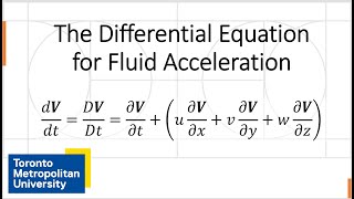
Detailed
In this section, we explore the intricacies of local acceleration within the context of fluid dynamics. Building on Newton's second law, we first establish that force is directly linked to mass and acceleration, leading to the computation of force at the particle level using the formula:
\[ F = m \cdot a \]
Here, acceleration is observed as the time derivative of particle velocity, which varies with respect to position and time, facilitating a deeper understanding through concepts like the Taylor series in multiple variables. The section further delineates between local acceleration—linked solely to time changes—and convective acceleration, caused by variations in velocity gradients across spatial coordinates. Examples demonstrate the practical calculations involved in determining the acceleration at given points, reaffirming that both local and convective accelerations are pivotal to analyzing fluid particle behavior and dynamics.
Youtube Videos

Audio Book
Dive deep into the subject with an immersive audiobook experience.
Understanding Acceleration in Fluids
Chapter 1 of 6
🔒 Unlock Audio Chapter
Sign up and enroll to access the full audio experience
Chapter Content
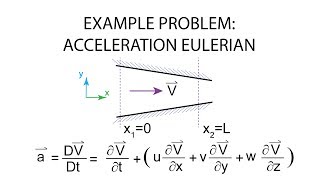
Now, let us look at the particle levels; if I had to find out what is the acceleration of the fluid particles? It is nothing else is a time derivative of velocity of the particles, as you know it from class 10, 11th and 12th I am just doing this time derivative of the velocity; particle velocities with respect to time and that is what represents the accelerations.
Detailed Explanation
In this chunk, we learn about how to determine the acceleration of fluid particles. Acceleration can be understood as the change in velocity over time. For fluid particles, this acceleration is calculated by taking the time derivative of the velocity, which is simply the rate of change of velocity with respect to time. This concept is fundamental to our understanding of flow dynamics as it allows us to quantify how quickly particles are accelerating or decelerating in a flow.
Examples & Analogies
Think of a car accelerating on a highway. When the driver steps on the gas pedal, the car's speed increases over time. By measuring how fast the speed changes, we’re effectively calculating the acceleration of the car, just like fluid particles accelerate based on their changing velocity.
Local Components of Acceleration
Chapter 2 of 6
🔒 Unlock Audio Chapter
Sign up and enroll to access the full audio experience
Chapter Content
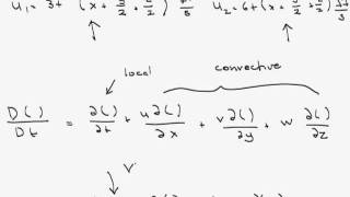
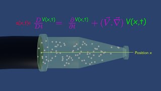
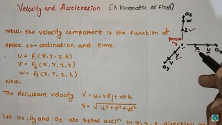
Now, if you look at this the velocities has a variability in a positions and the time because of that though when you define a; derivative with respect to time you will have a local component okay, you will have a with a x particle directions, y particle directions and z particle direction.
Detailed Explanation
This chunk discusses how acceleration can vary based on the position and time for fluid particles. It emphasizes that when we define acceleration as a derivative with respect to time, we need to consider the local components in different spatial dimensions (x, y, and z directions). These variations signify that particles may not only be accelerating but doing so in different directions, resulting in local acceleration components for each direction.
Examples & Analogies
Imagine an airplane flying through the sky. Depending on atmospheric conditions (like wind or turbulence), the plane may speed up (positive acceleration) or slow down (negative acceleration) in different directions based on its orientation. This scenario illustrates how local acceleration can vary across different axes.
Taylor Series and Acceleration
Chapter 3 of 6
🔒 Unlock Audio Chapter
Sign up and enroll to access the full audio experience
Chapter Content
This is nothing else if you are considering is a 2 variables like I just discussed you the Taylor series, if you remember it defining for the 2 variables. In this case, I have a Taylor series of 4 variables the x, y, z and the t. If you expand it and take it only these 4 terms, you will get this component nothing else, we are near to the same Taylor series concept.
Detailed Explanation
Here, the text introduces the concept of Taylor series and how it can be applied to understand acceleration in multi-dimensional fluid dynamics. The Taylor series allows us to approximate functions; in this case, we can extend it to include variables for position in three dimensions (x, y, z) and time (t). This mathematical approach helps in simplifying complex fluid behavior by focusing on a finite number of terms that contribute significantly to the acceleration.
Examples & Analogies
Consider baking a cake. If you want to predict how the cake will rise based on the ingredients you add (like eggs, flour, and sugar), you might start with a basic recipe (the initial value) and then apply adjustments (higher-order terms) based on how those ingredients influence the outcome. Similarly, in fluid dynamics, we can approximate how changes in position and time affect particle acceleration.
Components of Acceleration: Local and Convective
Chapter 4 of 6
🔒 Unlock Audio Chapter
Sign up and enroll to access the full audio experience
Chapter Content
These components change of the velocities is called convective or advective accelerations components, so this is 2 components; one is local acceleration component and other is convective acceleration.
Detailed Explanation
In this section, we differentiate between two types of acceleration in fluid dynamics: local acceleration and convective acceleration. Local acceleration refers to changes in velocity at a specific point in the flow over time, while convective acceleration relates to how fluid motion varies due to the movement of particles within the flow that influences their velocity profile. Both are crucial for understanding how particles behave in a dynamic fluid environment.
Examples & Analogies
Imagine riding a river's current. As you paddle forward (local acceleration), you also get swept along with the moving water (convective acceleration). Your speed changes not just because you're paddling, but also because of how fast the water is flowing around you.
Understanding Material Derivatives
Chapter 5 of 6
🔒 Unlock Audio Chapter
Sign up and enroll to access the full audio experience
Chapter Content
But many of the times people talk about material derivative, it is nothing else, it is that the change is a special name of the material derivative means, when you talk about a particles along the particles, you compute the derivative with respect to time is a total derivative or the material derivative or the particle derivatives.
Detailed Explanation
This part introduces material derivatives, which are a way of calculating how quantities change for a particle as it moves through a fluid. When we track a particle in a fluid (like a swimming fish), we examine how the properties of that particle evolve due to both the flow and its motion through space. Material derivatives thus articulate both local and convective effects experienced by particles.
Examples & Analogies
Think of a person walking through a crowded room. As they move forward, they might collide with other people, pushing them slightly out of their way. Here, the person's experience (material derivative) includes both their personal effort to walk forward and the interactions (like pushing) happening because others are moving around them.
Linking Eulerian and Lagrangian Observations
Chapter 6 of 6
🔒 Unlock Audio Chapter
Sign up and enroll to access the full audio experience
Chapter Content
So that is a breaching between these derivative component between the Eulerian frameworks and the Lagrangian frameworks. The virtual fluid ball concepts and that is what is link it as I said it.
Detailed Explanation
The final chunk emphasizes the connection between Eulerian and Lagrangian perspectives in fluid dynamics. Eulerian focuses on specific locations in the flow field to study velocity and acceleration at points, while Lagrangian tracks individual particles as they move through the fluid. This bridging allows for a comprehensive understanding of fluid behaviors by capturing both positional changes and particle-specific dynamics.
Examples & Analogies
Imagine watching a parade (Eulerian) from a fixed point versus being a participant walking alongside the parade (Lagrangian). The fixed observer sees how the parade moves over time, while the participant experiences the movement from within, gaining insights about both the overarching flow and individual elements.
Key Concepts
-
Newton's Second Law: The relationship between force, mass, and acceleration.
-
Local Acceleration: Change in velocity at a point with respect to time.
-
Convective Acceleration: Change in velocity due to spatial variation.
-
Taylor Series: A mathematical tool for estimating the values of functions at a point.
Examples & Applications
If a fluid particle has a velocity described by v = x^2 + y^2, the local acceleration can be defined by calculating the derivative of this velocity concerning time.
An example can also include analyzing how different velocities at the x, y, and z coordinates affect convective acceleration in a flowing fluid.
Memory Aids
Interactive tools to help you remember key concepts
Rhymes
If you want to know your flow, Check the force and let it show; Mass and acceleration in a dance; Together they’re the force — give it a chance!
Stories
Imagine a busy river where every drop of water is like a busy worker. Some drops speed up over time (local acceleration), while others speed up due to flowing into rapid parts of the river (convective acceleration).
Memory Tools
To remember Local and Convective: L in Local means 'Time' changes, C in Convective means 'Flow' changes.
Acronyms
LAC
Local Acceleration for Time
Convective for flow variation.
Flash Cards
Glossary
- Force
An interaction that causes an object to change its motion.
- Acceleration
The rate of change of velocity over time.
- Local Acceleration
Acceleration at a specific point in the fluid relating to time changes.
- Convective Acceleration
Acceleration caused by the spatial variation of velocity within the fluid.
Reference links
Supplementary resources to enhance your learning experience.