
Computing Acceleration
Enroll to start learning
You’ve not yet enrolled in this course. Please enroll for free to listen to audio lessons, classroom podcasts and take practice test.
Interactive Audio Lesson
Listen to a student-teacher conversation explaining the topic in a relatable way.
Introduction to Velocity Distribution
🔒 Unlock Audio Lesson
Sign up and enroll to listen to this audio lesson

Today, we're going to dive into velocity distributions, especially in converging nozzles. Can anyone tell me why velocity increases in a nozzle?

Is it because of the reduction in area?
Exactly! As area decreases, velocity increases based on the continuity equation. Now, let’s talk about how we define this velocity mathematically.

What's the equation for that?
Great question! The velocity distribution can be expressed as \( u = V_0(1 – \frac{L}{x}) \) or similar. Remember, V measures our initial velocity. Can anyone relate this to acceleration?

Acceleration would be the change in velocity over time!
Correct! This leads us to compute the acceleration's derivative. Let’s summarize: we’ve discussed the relationship between area and velocity and touched on acceleration.
Calculating Acceleration
🔒 Unlock Audio Lesson
Sign up and enroll to listen to this audio lesson

Now that we've understood the velocity components, let’s calculate acceleration. There are key components: local and convective acceleration.

What do we mean by local acceleration?
Local acceleration refers to how velocity changes with time at a specific point. Conversely, convective acceleration accounts for changes in velocity as you move through space. Both are essential in our analysis.
And how does that change in a steady flow?
In steady flow, the local acceleration becomes zero. Let’s recap what that means for our calculations.
Practical Examples
🔒 Unlock Audio Lesson
Sign up and enroll to listen to this audio lesson
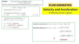
Let's solve a practical example to compute acceleration. If our velocity at entry is \(10 \text{ ft/s}\) and exit velocity is \(30 \text{ ft/s}\) over certain lengths, what’s our strategy?
We substitute those values into our derivative equation?
Absolutely! You’ll find the acceleration at each point. Remember, the flow is steady, so local acceleration is zero, simplifying our math. Can anyone calculate what their value would be?
The acceleration would equal the change in velocity over distance!
Exactly! Repeat this process for various flows, and you’ll gain more insight. Let’s summarize our calculations.
Application in Fluid Dynamics
🔒 Unlock Audio Lesson
Sign up and enroll to listen to this audio lesson
Now, let’s discuss why computing acceleration is crucial in fluid dynamics.
It helps in predicting how fluids will move in different systems!
Spot on! And remember, these principles apply to various real-world scenarios, like in designing jet engines or nozzles.
So these computations help engineers design better equipment?
Exactly! Understanding acceleration allows for optimized designs, improving efficiency and safety. To summarize, we covered definitions, calculations, and applications. Any further questions for clarification?
Introduction & Overview
Read summaries of the section's main ideas at different levels of detail.
Quick Overview
Standard
The section explores the computation of acceleration within a 1-dimensional fluid flow scenario, specifically in converging nozzles. It emphasizes the total derivative of velocity, local accelerations, and their relation to the convective acceleration components, with a focus on steady flow conditions. The topic concludes with example problems illustrating the application of theory to practical situations.
Detailed
Detailed Summary
This section focuses on the computation of acceleration in fluid dynamics, particularly in scenarios involving converging nozzles where the fluid flow is one-dimensional. It begins with an examination of velocity components at the entrance and exit points of a nozzle and moves on to derive the acceleration equations.
Key Concepts
- Velocity Distribution: The section introduces the velocity distribution formula and how it varies from entry to exit in a converging nozzle.
- Acceleration Calculation: The acceleration in the x-direction, represented as
du/dt, is computed using the total derivative method. It also elaborates on the distinction between local accelerations and convective accelerations. - Steady Flow Considerations: The discussion emphasizes the conditions of steady flow, resulting in simplifications where certain components equal zero, making calculations easier.
- Example Problems: Finally, example calculations clarify the theoretical components, illustrating real-world applications of these principles in determining acceleration based on given parameters.
Overall, this section is vital for understanding the fundamental principles of fluid dynamics related to acceleration computation.
Youtube Videos


Audio Book
Dive deep into the subject with an immersive audiobook experience.
Understanding Velocity and Acceleration
Chapter 1 of 5
🔒 Unlock Audio Chapter
Sign up and enroll to access the full audio experience
Chapter Content
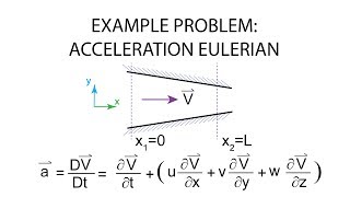
And at the entrance points and the velocity at the exit point will be the 3. And the velocity distributions is given with respect to the x directions this is the about the nozzles. The velocity field is given as:
\[ V = 2 \pi \sqrt{\text{some value}} \cdot u_1 \cdot g \cdot x \cdot L \cdot \text{other variables} \]
This is what the velocity distributions given to us. What we have to need to compute it? What is the acceleration in the x directions? du/dt at the entrance point at this x = 0 that is what the entrance and this is what of exit of the flow.
Detailed Explanation
At the start and end of a flow process in a nozzle, we look at how fast the fluid is moving. This movement is described as 'velocity,' which varies along the length of the nozzle. The given equation indicates how the velocity changes, depending on certain parameters like position (x) and others related to the nozzle dynamics. To find acceleration, we need to know how velocity changes over time (du/dt).
Examples & Analogies
Imagine a water slide: at the top (entrance), water moves slowly, and at the bottom (exit), it speeds up. The change in speed (velocity) as it slides down is what we're measuring as acceleration.
Calculating Acceleration Components
Chapter 2 of 5
🔒 Unlock Audio Chapter
Sign up and enroll to access the full audio experience
Chapter Content
So if it is the conditions we need to compute it what will be the accelerations ax du/dt. If the \( u = 10 \text{ ft/s} \) and the length is 1 feet. Now if you look at these problems is very easy problems it may be has described as the converging nozzles giving the velocity increase of the velocity as the nozzle dimension is coming, decreasing trend.
Detailed Explanation
Here, we want to determine the acceleration (ax) at the entrance to the nozzle using the equation ax = du/dt (change of velocity per time). Given that the initial velocity (u) at one point is 10 feet/second, we can calculate how much this velocity changes as the fluid passes through the nozzle.
Examples & Analogies
Think of a car accelerating from 0 to 60 mph. The change in speed as the car moves down the road is similar to what we're examining in the nozzle – we are trying to find out how rapidly the speed is changing.
Steady Flow Considerations
Chapter 3 of 5
🔒 Unlock Audio Chapter
Sign up and enroll to access the full audio experience
Chapter Content
But if you look at these problems what are the components can be neglected as it is a steady flow there is no time component on this. We can make it this is equal to 0 and since it is a 1 dimensional flow as it is a steady flow when is no time component in the velocity field and it is a 1 dimensional flow.
Detailed Explanation
In a steady flow scenario, the speed of the fluid does not change with time at any particular point, meaning terms related to 'du/dt' can be treated as zero. This simplifies our calculations. The '1-dimensional flow' suggests that we are only considering changes in one direction, which also makes the calculations easier.
Examples & Analogies
Consider a river flowing at a constant speed in a straight path. If the flow rate remains the same, we don't need to account for changes over time – we can just focus on how the river moves in that singular direction.
Calculating Specific Accelerations
Chapter 4 of 5
🔒 Unlock Audio Chapter
Sign up and enroll to access the full audio experience
Chapter Content
So if you just substitute this value and do a partial derivative of this u with respect to x and if you substitute it will get it the du that by substitute it is:
\[ \frac{du}{dx} \text{ value} \]
So it is very easy as you do a partial derivative with respect to x. If you do the partial derivative you can look it and substituting this the u value, you will get this value.
Detailed Explanation
We can calculate the acceleration by taking the derivative of our initial velocity equation concerning the position (x). This derivative gives us information about how velocity changes as we move along the nozzle, allowing us to conclude about acceleration at specific points.
Examples & Analogies
Imagine measuring the slope of a hill: the steepness at any point can tell you how fast something would roll down. The derivative of our velocity with respect to position (x) serves a similar purpose to measure changes in speed.
Finalizing Calculations at Specific Points
Chapter 5 of 5
🔒 Unlock Audio Chapter
Sign up and enroll to access the full audio experience
Chapter Content
So we know this how this accelerations ax varies with respect to x and what is a functions in terms of V and the L? So we have to find out what will be the velocity when x = 0 and x = L and the \( V_0 \) is given to us. So using given data we can compute it the accelerations in the x directions du/dt at x = 0. I am just substitute it in here when x = 0.
Detailed Explanation
Now, we need to calculate specific acceleration values at defined points in our nozzle, notably at the starting point (x = 0) and the endpoint (x = L). Substituting these x-values into our acceleration equations allows us to find out exactly how fast the fluid is accelerating in these regions.
Examples & Analogies
Consider a car taking off from a stoplight; knowing the speed when the light turns green (x = 0) and how fast it's speeding up by the time it crosses a junction (x = L) give us key insights into its acceleration.
Key Concepts
-
Velocity Distribution: The section introduces the velocity distribution formula and how it varies from entry to exit in a converging nozzle.
-
Acceleration Calculation: The acceleration in the x-direction, represented as
du/dt, is computed using the total derivative method. It also elaborates on the distinction between local accelerations and convective accelerations. -
Steady Flow Considerations: The discussion emphasizes the conditions of steady flow, resulting in simplifications where certain components equal zero, making calculations easier.
-
Example Problems: Finally, example calculations clarify the theoretical components, illustrating real-world applications of these principles in determining acceleration based on given parameters.
-
Overall, this section is vital for understanding the fundamental principles of fluid dynamics related to acceleration computation.
Examples & Applications
Example 1: Calculating accelerations at the entrance and exit of a converging nozzle by substituting velocity values into the derived equations.
Example 2: Evaluating the velocity field using given parameters to determine accelerations in a steady-state flow.
Memory Aids
Interactive tools to help you remember key concepts
Rhymes
When velocity climbs at the nozzle’s tight bend, acceleration follows, on this we depend.
Stories
Imagine a funnel, water pouring in. As it narrows, the speed builds—just like our fluid flow!
Memory Tools
To remember fixed flow properties, think 'Steady: No Change, Steady: No Danger!'
Acronyms
VACC
Velocity
Acceleration
Change
Convective—four key concepts connecting fluid dynamics.
Flash Cards
Glossary
- Velocity Distribution
The variation of flow velocity within a cross-section of a nozzle or channel.
- Local Acceleration
The change in velocity at a specific point in the flow field over time.
- Convective Acceleration
The change in velocity due to motion through the flow field, observed over a spatial domain.
- Steady Flow
A flow condition where fluid properties at a point do not change with time.
Reference links
Supplementary resources to enhance your learning experience.