
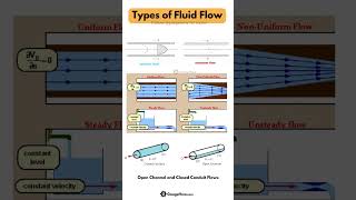
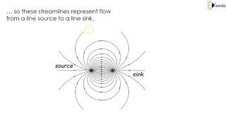
Fluid Particle Direction in Dipole Source Flow
Enroll to start learning
You’ve not yet enrolled in this course. Please enroll for free to listen to audio lessons, classroom podcasts and take practice test.
Interactive Audio Lesson
Listen to a student-teacher conversation explaining the topic in a relatable way.
Understanding Velocity Distributions
🔒 Unlock Audio Lesson
Sign up and enroll to listen to this audio lesson

Let's start with the velocity distributions in fluid flows, particularly in nozzles. Who can tell me how velocity changes as it travels through a nozzle?

I think the velocity increases as the cross-section decreases.
Exactly! This phenomenon is described by the continuity equation. In our equation, we find that velocity at the exit point can be three times that at the entrance. Remember this term: 'continuity' establishes that mass flow rate remains constant.

What does that mean for the acceleration of fluid particles?
Great question! The acceleration can be computed by considering the changes in velocity. Specifically, we calculate the total derivative of the velocity concerning time in the x-direction. Now, can anyone recall why simplifying assumptions can lead to some components being neglected?

Because it’s a steady flow, right? So, components with time variations can be set to zero.
Exactly right! As it’s steady, those terms drop out. Let’s summarize: velocity increases due to converging nozzles, and acceleration is calculated through derivatives that ignore time-dependent components.
Acceleration Calculations
🔒 Unlock Audio Lesson
Sign up and enroll to listen to this audio lesson

Next, let’s compute accelerations at various coordinates along the flow. We know the exit velocity at x equals L; how do we find acceleration at points x=0 and x=L?
We substitute our values for velocity into the acceleration formula, right?
Precisely! When x equals 0, if we substitute our known values, what acceleration do we find?

It should yield 200 feet per square second.
Correct! And at the exit point x=L, we find it increases to 600 feet per square second. What can we infer about the system based on these results?
The acceleration increases as fluid moves through the nozzle, which supports the increase in velocity.
Excellent! Let’s remember: as fluid accelerates in a converging nozzle, both velocity and acceleration grow.
Streamlines and Acceleration in 2D Flow
🔒 Unlock Audio Lesson
Sign up and enroll to listen to this audio lesson
Now, let’s transition from one-dimensional to two-dimensional flow. How does understanding streamlines change our approach to fluid dynamics?
Streamlines give us a visual representation of flow patterns, right? We can see how fluid particles move.
Exactly! When dealing with streamlines, we use stream functions. What is the mathematical relationship we maintain?
The slope of the streamline equals Vy/Vx, indicating the angle of flow.
Correct! So when we evaluate a streamline, we can derive equations such as for hyperbolic shapes. What's our next step?
We calculate the acceleration by differentiating the velocity components with respect to time.
Right again! So, let’s summarize: streamlines allow us to visualize flow; knowing slope relationships is vital for computing particle acceleration in a defined flow field.
Practical Applications and Examples
🔒 Unlock Audio Lesson
Sign up and enroll to listen to this audio lesson
Let’s discuss how these concepts apply in practical scenarios. Can anyone provide an example where knowing fluid acceleration is vital?
In designing jets or engines, we need to know how fast the fluid is accelerating.
Exactly! Accelerations will determine thrust forces and overall system efficiency. How does this relate to the earlier examples we calculated?
The exit velocity and increase in acceleration are essential for optimizing design.
Yes! Each design aspect, from nozzle shape to exit velocity, will impact functionality. As a recap: understanding acceleration and velocity in fluid dynamics is crucial for practical applications.
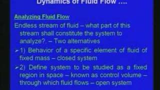
Introduction & Overview
Read summaries of the section's main ideas at different levels of detail.
Quick Overview
Standard
In this section, we explore fluid dynamics related to dipole source flows, particularly how fluid particles behave within a nozzle's constriction and the resulting acceleration. The equations governing velocity distribution and acceleration calculations are introduced, concluding with examples to deepen understanding.
Detailed
Fluid Particle Direction in Dipole Source Flow
This section examines the behavior of fluid particles in a dipole source flow and investigates how their velocity and acceleration are computed at specific points. It begins by outlining the velocity field represented in one-dimensional terms, particularly focusing on nozzle dynamics where the velocity increases as the nozzle constricts. The mathematical formulation provided leads to calculating the acceleration in the x-direction as a total derivative of the velocity component with respect to time. The section highlights that for steady flows, certain components of acceleration can be neglected, simplifying computations significantly.
In illustration, examples are given where the velocities at the entrance and exit points of a nozzle are derived, facilitating the understanding of particle acceleration as the nozzle dimensions change. Following this, the section delves into a two-dimensional flow field, reinforcing the concept of streamline patterns and allowing for the exploration of more complex dynamics at given x and y coordinates. Various equations such as those for stream functions provide valuable insights into the overall behavior of fluid particles in this context.
Youtube Videos


Audio Book
Dive deep into the subject with an immersive audiobook experience.
Understanding Fluid Velocity and Acceleration
Chapter 1 of 6
🔒 Unlock Audio Chapter
Sign up and enroll to access the full audio experience
Chapter Content
And at the entrance points and the velocity at the exit point will be the 3 . And the velocity distributions is given with respect to the x directions this is the about the nozzles.
Detailed Explanation
In this section, we are discussing fluid velocity and acceleration. The velocities at the entrance and exit points of a nozzle are important parameters in fluid mechanics. The velocities are often given in a mathematical form, illustrating how they change with respect to their position in the flow path. In this case, the focus is on how the velocity increases as the nozzle dimensions decrease, which is a common feature in fluid flow through nozzles.
Examples & Analogies
Imagine a garden hose: when you place your thumb over the end of the hose, the water shoots out faster because the diameter is narrower. This is similar to what happens in a nozzle where the fluid accelerates as the space it can flow through gets smaller.
Calculating Accelerations in Fluid Flow
Chapter 2 of 6
🔒 Unlock Audio Chapter
Sign up and enroll to access the full audio experience
Chapter Content
What we have to need to compute it? What is the acceleration in the x directions? du/dt at the entrance point at this x = 0 that is what the entrance and this is what of exit of the flow.
Detailed Explanation
To compute the acceleration of fluid flow, we need to evaluate the change in velocity over time at certain points. In this case, we are looking at the entrance and exit points within the fluid dynamics context. The acceleration is defined as the total derivative of the velocity component concerning time, focusing on the x-direction. This derivative captures both local and convective accelerations, allowing us to analyze how fast the fluid is speeding up as it moves.
Examples & Analogies
Think about how a car accelerates on a highway. When the driver presses the accelerator pedal, the car's velocity increases over time, just like how the velocity of fluid particles increases as they pass through the constricted part of the nozzle.
Impact of Steady Flow on Acceleration Components
Chapter 3 of 6
🔒 Unlock Audio Chapter
Sign up and enroll to access the full audio experience
Chapter Content
But if you look at these problems what are the components can be neglected as it is a steady flow there is no time component on this.
Detailed Explanation
In steady flow, the fluid's velocity at any given point does not change over time. Therefore, certain components of acceleration that depend on the time derivative can be considered zero. This simplification makes calculations easier since we can focus on the spatial variations of velocity rather than how that velocity changes over time.
Examples & Analogies
Consider a river flowing steadily in one direction. If the flow is constant, you wouldn't expect the speed of the flowing water to change at any given spot over time, which means you can analyze it as if it were not changing.
Substituting Values to Find Acceleration
Chapter 4 of 6
🔒 Unlock Audio Chapter
Sign up and enroll to access the full audio experience
Chapter Content
So it is quite easy we have to compute this part. So if you just substitute this value and do a partial derivative of this u with respect to x.
Detailed Explanation
To find the acceleration at different positions in the flow, we substitute the values into our equations and perform a partial derivative with respect to spatial position, x. This allows us to see how the velocity changes across the nozzle, providing insights into how fluid accelerates as it moves through this constriction.
Examples & Analogies
If you want to find out how fast a bike is going when you start pedaling harder, you would measure the speed at different points along your path. Similarly, we look at the velocity at different points in the nozzle to understand the behavior of the fluid.
Accelerations at Specific Points
Chapter 5 of 6
🔒 Unlock Audio Chapter
Sign up and enroll to access the full audio experience
Chapter Content
So using given data we can compute it the accelerations in the x directions du/dt at x = 0.
Detailed Explanation
After substituting the given values, we calculate the acceleration at specific points—here at x = 0 and x = L. This helps us determine how the fluid's speed changes at the beginning and the end of the nozzle, illustrating the acceleration profile throughout the nozzle.
Examples & Analogies
Think of it as measuring the speed of a runner at the start and the finish line of a race. By knowing their speed at those two points, we can infer how much they accelerated throughout the course.
Summary of Findings in Fluid Acceleration
Chapter 6 of 6
🔒 Unlock Audio Chapter
Sign up and enroll to access the full audio experience
Chapter Content
So let me summarize these problems one of the easy problems only it has described the velocity field giving a converging nozzles and telling this the velocity at this point is equal to V and the 0 velocity increases into 3 times of V here.
Detailed Explanation
To summarize, we have analyzed the fluid velocity and acceleration within a converging nozzle. The findings illustrate that as the fluid passes through, its velocity increases significantly up to three times its initial value at the exit point of the nozzle.
Examples & Analogies
Like a dancer transitioning from a slow movement to a swift spin, fluid flows rapidly through the nozzle, showcasing an increase in speed as it narrows down before exiting.
Key Concepts
-
Velocity Increase: Fluid velocity increases through a nozzle's constricted area.
-
Acceleration Calculation: Acceleration is determined by the total derivative of velocity concerning time.
-
Steady Flow Assumption: In steady flow, time-dependent acceleration components can be neglected.
-
Streamlines Visualization: Streamlines visually represent the flow direction and are critical for analyzing fluid dynamics.
Examples & Applications
Example 1: Calculating acceleration at entrance and exit points of a nozzle setup.
Example 2: Illustrating 2D flow patterns using stream functions.
Memory Aids
Interactive tools to help you remember key concepts
Rhymes
In a narrow nozzle, watch the rush, fluid speeds, oh what a hush!
Stories
Imagine a river where rocks create eddies; the water speeds up as it flows through narrow spaces. Just like this river, fluid accelerates in nozzles!
Memory Tools
For velocity, remember: Nozzles Increase Speed (NIS).
Acronyms
STEADY
Steady Time Effects Are Dismissed Yielding - No flow change.
Flash Cards
Glossary
- Velocity Distribution
The variation of speed at various points in a fluid flow, especially in nozzles.
- Acceleration
The rate of change of velocity of fluid particles, critical to understanding fluid behaviors.
- Streamline
A curve that is everywhere tangent to the velocity field, illustrating fluid flow direction.
- Steady Flow
A flow condition where fluid properties at a point do not change with time.
Reference links
Supplementary resources to enhance your learning experience.