
Computing Accelerations in 2D Flow
Enroll to start learning
You’ve not yet enrolled in this course. Please enroll for free to listen to audio lessons, classroom podcasts and take practice test.
Interactive Audio Lesson
Listen to a student-teacher conversation explaining the topic in a relatable way.
Understanding Velocity Distributions
🔒 Unlock Audio Lesson
Sign up and enroll to listen to this audio lesson

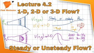
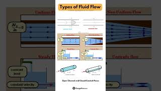
Today, we begin by discussing velocity distributions in a 2D flow, which are crucial for understanding acceleration.

What exactly do we mean by velocity distributions?
Great question! Velocity distributions refer to how the velocity varies across different points in the flow field. In nozzles, for example, as the cross-sectional area reduces, the velocity increases.

So velocity at different points matters for calculating acceleration?
Exactly! To compute acceleration, we look at both local and convective acceleration components, which depend on these velocity distributions.

How do we actually calculate those accelerations?
We take the total derivative of the velocity with respect to time, considering each component's contributions.
Can you give us a formula for that?
Absolutely! The acceleration in the x-direction, for instance, can be derived using partial derivatives of velocity with respect to time and space.
To summarize, velocity distributions vary with flow conditions and are critical to computing accelerations accurately.
Local and Convective Accelerations
🔒 Unlock Audio Lesson
Sign up and enroll to listen to this audio lesson

Let's build on our earlier discussion and delve into local and convective accelerations.
What’s the difference between local and convective acceleration?
Good question! Local acceleration refers to the change of velocity at a point over time, while convective acceleration is related to changes due to motion through a velocity field.

How do we express these mathematically?
Mathematically, local acceleration can be expressed as the partial derivative of velocity with respect to time, while convective acceleration involves spatial derivatives.
What do we usually neglect in steady flows?
In steady flows, we can often neglect time-dependent components, simplifying our calculations.
To wrap up, remember that local and convective accelerations help us understand how fluid motion changes in a 2D flow.
Practical Example: Converging Nozzles
🔒 Unlock Audio Lesson
Sign up and enroll to listen to this audio lesson
Now let’s apply what we’ve learned through a practical example involving converging nozzles.
What exactly will we be calculating?
We will calculate accelerations at the entrance and exit points of the nozzle using given velocity distributions.
How do we approach this computation?
We substitute values from the velocity distributions into our derived formulas for acceleration.
Can we get numerical answers from this?
Yes! By substituting specific values, we can compute acceleration at various points, revealing how it varies across the nozzle.
So, to summarize, applying practical examples enriches our understanding of both theoretical concepts and real-world applications of fluid flows.
Computing Accelerations Around Circular Cylinders
🔒 Unlock Audio Lesson
Sign up and enroll to listen to this audio lesson
Next, let's discuss flow around circular cylinders and how we compute accelerations in this context.
What is the significance of studying flow around cylinders?
Studying flow around cylinders helps in understanding concepts like drag, lift, and vortex formation.
How do we establish the velocity field in this case?
The velocity field can be established using stream functions, considering the axisymmetric nature of the flow.
What happens to the radial velocity component?
Great observation! The radial component is typically zero at the surface of the cylinder due to the no-slip condition.
To conclude, recognizing how flows interact with cylindrical structures informs both theoretical and practical aspects of fluid dynamics.
Introduction & Overview
Read summaries of the section's main ideas at different levels of detail.
Quick Overview
Standard
In this section, we explore how to compute accelerations in 2-dimensional flow, particularly through continuous examples involving nozzles and circular cylinders. The acceleration is derived from the velocity distributions, emphasizing local and convective acceleration components, as well as practical approaches to simplifying computations under steady flow conditions.
Detailed
In this section, we delve into the mathematical framework for computing accelerations within a two-dimensional flow field. The section begins with a brief look at velocity distributions relevant to nozzles, illustrating the relationship between velocity and acceleration at both entrance and exit points of the flow. We define accelerations as the total derivative of velocity with respect to time, addressing both local and convective acceleration components, particularly within the x-direction. Further, through detailed examples—gradually increasing in complexity—we analyze flow around converging nozzles and circular cylinders. Numerical computations highlight practical applications and assumptions under steady flow conditions, enabling simplifications in determining acceleration outputs. Drawing from figures and equations, the section equips readers with the tools needed to understand the dynamics of fluid motion in two-dimensional spaces.
Youtube Videos


Audio Book
Dive deep into the subject with an immersive audiobook experience.
Introduction to the Problem
Chapter 1 of 6
🔒 Unlock Audio Chapter
Sign up and enroll to access the full audio experience
Chapter Content
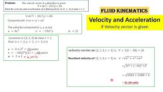
The velocity distributions is given with respect to the x directions this is about the nozzles. The velocity field is given as the 2\pi \sqrt{y} V_1.
Detailed Explanation
In this section, we start by discussing the velocity distribution in a two-dimensional flow, particularly as it pertains to nozzles. The velocity field is defined mathematically to help us understand how the velocity varies in the x-direction. The expression '2π√y V_1' represents the velocity field where 'V_1' is the velocity at a specified point.
Examples & Analogies
Imagine a garden hose that narrows at the nozzle. As you squeeze the nozzle, the water flows faster – this is similar to how the velocity increases in a converging nozzle in fluid dynamics.
Computing Acceleration (du/dt)
Chapter 2 of 6
🔒 Unlock Audio Chapter
Sign up and enroll to access the full audio experience
Chapter Content
We need to compute it. What is the acceleration in the x directions? du/dt at the entrance point at x = 0.
Detailed Explanation
To find the acceleration in the x-direction (denoted as du/dt), we first look at the entrance point where x = 0. This is significant because the behavior of the fluid at the entrance provides valuable information about how it will flow and change. This step is crucial in fluid dynamics to calculate how fast the flow changes over time.
Examples & Analogies
Think of a car at a traffic light. When the light turns green (the entrance point), you accelerate from a stop. This acceleration changes based on how fast you're pressing the gas pedal, which is similar to how the fluid's velocity changes over time.
Acceleration in Steady Flow
Chapter 3 of 6
🔒 Unlock Audio Chapter
Sign up and enroll to access the full audio experience
Chapter Content
If it is steady flow, there is no time component on this. We can make it this is equal to 0.
Detailed Explanation
In steady flow, conditions do not change over time. Therefore, when we calculate the acceleration, we find that time derivatives can be disregarded (equal to zero). This simplifies our calculations, as we only need to assess the spatial gradient of velocity.
Examples & Analogies
Consider the flow of a river where the water level and speed are constant. Just like the river's flow remains steady, the fluid in our analysis has a consistent flow pattern during the observation.
Calculating the Partial Derivative
Chapter 4 of 6
🔒 Unlock Audio Chapter
Sign up and enroll to access the full audio experience
Chapter Content
So it is very easy as you do a partial derivative with respect to x. If you do the partial derivative, you can look it and substituting this the u value, you will get this value.
Detailed Explanation
To calculate how the velocity 'u' changes concerning the x-direction, we perform a partial derivative. This mathematical operation helps us determine localized rates of change within the flow, which is essential for understanding variations in fluid motion.
Examples & Analogies
Think of a water flow in a pipe with varying diameters. By measuring how the water pressure changes at different points in the pipe, we gain insights into the fluid's behavior as it flows through these varying sections.
Acceleration at Different Points
Chapter 5 of 6
🔒 Unlock Audio Chapter
Sign up and enroll to access the full audio experience
Chapter Content
At entrance point (x = 0) the acceleration is 200 feet/s² and at exit point (x = L), the acceleration is 600 feet/s².
Detailed Explanation
After computing the acceleration in different locations, we find distinct values at the entrance and exit points of the flow. At x = 0, the acceleration is calculated to be 200 feet/s², while at x = L, it rises to 600 feet/s². This indicates that as the fluid flows through the nozzle, it speeds up significantly.
Examples & Analogies
Returning to our garden hose, if you measure how quickly the water accelerates when you move from the wider part of the hose to the narrower part, you'd see similar acceleration changes reflecting the calculations we've made.
Summary of the Computation of Accelerations
Chapter 6 of 6
🔒 Unlock Audio Chapter
Sign up and enroll to access the full audio experience
Chapter Content
Summary of problems one of the easy problems... velocity field giving a converging nozzles...
Detailed Explanation
In this summary, we encapsulate the essence of the computations regarding the acceleration in our two-dimensional flow. It emphasizes that understanding how velocity changes from one point to another in a nozzle is critical in fluid dynamics, and these calculations can help predict future behaviors of fluid in similar systems.
Examples & Analogies
Consider how an expert chef adjusts the heat on a stove to ensure the food cooks evenly. Similarly, engineers use these computations to adjust flow dynamics in applications, ensuring they operate efficiently and effectively.
Key Concepts
-
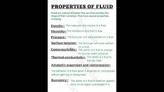
Velocity Distributions: The variation of fluid velocity at different points in a flow.
-
Local Acceleration: Change in velocity at a given point over time.
-
Convective Acceleration: Change in velocity due to the movement through differing velocity fields.
-
Steady Flow Simplifications: Under steady conditions, certain components can be disregarded for calculations.
Examples & Applications
Example of calculating accelerations in a nozzle flow with given velocity distributions.
Illustration of flow around a circular cylinder and its impact on velocity fields.
Memory Aids
Interactive tools to help you remember key concepts
Rhymes
In flows where velocities change, Acceleration’s task isn’t strange.
Stories
Imagine a water slide where a ball accelerates faster as it goes downhill; it mimics how fluid velocities change in a real flow field.
Memory Tools
A-C-L: Acceleration, Convective, Local helps to remember the types of accelerations in fluid flow.
Acronyms
FLAB
Flow
Local
Acceleration
Boundaries - a way to remember key concepts in fluid dynamics.
Flash Cards
Glossary
- Acceleration
The rate of change of velocity with respect to time.
- Local Acceleration
The change in velocity at a specific point over time.
- Convective Acceleration
The change in velocity due to the movement of the fluid through spatial variations in velocity.
- Velocity Distribution
The variation of fluid velocity at different points in space.
- Steady Flow
A flow condition where fluid properties at any point do not change with time.
Reference links
Supplementary resources to enhance your learning experience.