
Sketching of Streamlines
Enroll to start learning
You’ve not yet enrolled in this course. Please enroll for free to listen to audio lessons, classroom podcasts and take practice test.
Interactive Audio Lesson
Listen to a student-teacher conversation explaining the topic in a relatable way.
Understanding Velocity Distributions
🔒 Unlock Audio Lesson
Sign up and enroll to listen to this audio lesson

Today, we will start with understanding velocity distributions in converging nozzles. Can anyone tell me what a velocity distribution is?

Isn't it how the speed of the fluid varies at different points?
Exactly! In converging nozzles, as the cross-section decreases, the fluid accelerates. This change in velocity is described by a specific equation. Remember: 'As the nozzle narrows, speed up!' — that could be a good mnemonic!

So, how do we find the acceleration from this velocity distribution?
Great question! We can calculate the acceleration along the x-direction using the partial derivative of velocity with respect to time. Simply put, it involves some calculus to find how speed changes along the streamline.
Calculating Accelerations
🔒 Unlock Audio Lesson
Sign up and enroll to listen to this audio lesson

Now, let's dive deeper into calculating acceleration. At the entrance and exit of the flow, we can derive specific values by substituting known velocities. Who can tell me what happens to the time component in a steady flow?

I think it becomes zero because there’s no change over time!
Correct! In steady flow, time derivatives vanish. Hence, the acceleration simplifies to a function of spatial variables only. Let’s illustrate how we can compute these changes with specific values.

Are the acceleration values the same at different points within the nozzle?
Good point! No, they vary. For instance, at x=0, there’s an acceleration related to the initial velocity, and at the exit point, it can be three times greater!
Stream Functions in Two-Dimensional Flow
🔒 Unlock Audio Lesson
Sign up and enroll to listen to this audio lesson
Moving on, let's talk about stream functions in two-dimensional flow. Stream functions help visualize flow patterns. Can anyone define them?
Are they functions that represent the flow of fluid without direct reference to time?
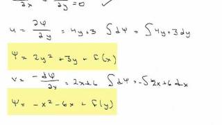
Exactly! They allow us to sketch streamlines that illustrate how fluid moves. The slope of the streamline relates to the velocity components. Anyone remember how to derive the equation for these components?
Isn’t it based on the partial derivatives of velocity functions?
Correct! Once we plot streamlines, we can derive acceleration fields as well. Always remember: 'Streamlines guide the flow!' That’s a good mnemonic too!
Practical Application - Example Problems
🔒 Unlock Audio Lesson
Sign up and enroll to listen to this audio lesson
Finally, let’s look at some practical examples to cement our understanding. Can someone explain how to derive the streamline pattern for our flow field?
I think we use the velocity equations to determine the corresponding stream functions?
Absolutely! Once you have the equations set, sketching the streamlines will involve integration. What do we expect to see in a flow around a cylinder?
We would see circular streamlines around it!
Right! The flow behaves predictably in predictable patterns. This reinforces the importance of understanding each element we discussed. Remember to keep practicing these calculations!
Introduction & Overview
Read summaries of the section's main ideas at different levels of detail.
Quick Overview
Standard
In this section, we explore the velocity distribution in one-dimensional flow, particularly through converging nozzles, and how to compute the resulting accelerations at various points in the flow. Key concepts include the relationship between velocity and acceleration components, and the significance of stream functions for understanding flow behavior.
Detailed
Detailed Summary
In this section, we focus on the concept of streamlines and how to sketch them based on the velocity distribution in fluid flow systems, specifically when dealing with converging nozzles. The velocity field is defined mathematically, and its behavior at entry and exit points is analyzed.
Key concepts include:
- The computation of acceleration components in the x-direction as flow progresses through a nozzle.
- Understanding velocity distributions and their impact on the fluid dynamics, exemplified by the local velocity at different points in a converging nozzle.
- The simplification associated with steady flows where temporal changes can be neglected.
- The definitions and applications of stream functions in two-dimensional flow, leading to the derivation of accelerations based on scalar components.
The section concludes with practical examples, illustrating how to visualize and analyze streamline patterns through mathematical formulations. This understanding is crucial for predicting flow behaviors in engineering applications.
Youtube Videos
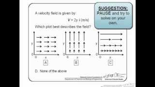
![Streamline Equation: Example 2 [Fluid Mechanics #7]](https://img.youtube.com/vi/sbT83oSbliA/mqdefault.jpg)

Audio Book
Dive deep into the subject with an immersive audiobook experience.
Introduction to Velocity Distributions
Chapter 1 of 4
🔒 Unlock Audio Chapter
Sign up and enroll to access the full audio experience
Chapter Content
The velocity distributions is given with respect to the x directions this is the about the nozzles. The velocity field is given as the \[ V = 2\sqrt{y} - \frac{4}{3} \] which indicates how velocity varies in x direction with respect to the nozzle geometry. At the entrance, we consider the velocity and the conditions to compute acceleration in the x direction, \( du/dt \).
Detailed Explanation
This chunk introduces the concept of velocity distributions, particularly how they vary in a nozzle. Here, the velocity field's equation shows how the flow changes with the nozzle's geometry. It emphasizes the need to calculate accelerations at specific flow points where the fluid enters the nozzle, which is crucial for understanding the nozzle dynamics.
Examples & Analogies
Think of running water through a garden hose: as you pinch the end of the hose, the velocity increases because the water is forced through a smaller opening. This illustrates how a nozzle's geometry affects water speed.
Understanding Acceleration in Flow
Chapter 2 of 4
🔒 Unlock Audio Chapter
Sign up and enroll to access the full audio experience
Chapter Content
We need to compute accelerations in the x direction, \( a_x = \frac{du}{dt} \), particularly at entrance and exit points. If the velocity at the entrance is 10 ft/s and the length is 1 ft, we find these accelerations as derivatives of the flow velocity with respect to time.
Detailed Explanation
This chunk delves deeper into calculating the acceleration in fluid flow. The acceleration component is defined as how velocity changes over time. By analyzing the velocity at specific points (the entrance and exit of the nozzle), we can evaluate how quickly the flow speed is changing, which is essential for predicting flow behavior in the nozzle.
Examples & Analogies
Consider a car accelerating: if the driver presses the gas pedal, the speed of the car increases over time. Similarly, in fluid dynamics, if the fluid's velocity increases as it flows through a nozzle, that change in speed represents acceleration.
Calculating Partial Derivatives for Acceleration
Chapter 3 of 4
🔒 Unlock Audio Chapter
Sign up and enroll to access the full audio experience
Chapter Content
The acceleration in the x direction can also be computed using the total derivative of the velocity component with respect to time, expressed as a partial derivative to account for steady flow conditions.
Detailed Explanation
Here, we focus on the mathematical aspect of calculating flow acceleration using partial derivatives. This is important in steady flow, where the velocity does not change over time, meaning that we can simplify some components of our calculations. The chunk explains that under certain conditions (steady and one-dimensional flow), the time derivatives can be considered zero, simplifying the process significantly.
Examples & Analogies
Picture a train moving steadily along a track; if no external forces act on it, its speed remains constant despite time passing. In fluid dynamics, when conditions are stable, we can disregard any time-related changes in velocity.
Final Acceleration at Entrance and Exit Points
Chapter 4 of 4
🔒 Unlock Audio Chapter
Sign up and enroll to access the full audio experience
Chapter Content
After substituting values for velocity and length into our equations, we find the accelerations at the entrance point and exit point. The result shows that the acceleration increases in the flow direction.
Detailed Explanation
This segment summarizes the results of our calculations. By substituting specific flow values into the equations derived earlier, we can determine real acceleration values at both the entrance and the exit of the nozzle. This highlights how acceleration changes from the start to the end of the flow path, demonstrating the physical behavior of the fluid within the system.
Examples & Analogies
Like a roller coaster that accelerates down a slope, the nozzle also shows how fluid accelerates due to the pressure and geometry. At the beginning, the flow has one speed, but as it pushes through the constriction of the nozzle, it speeds up, similar to a coaster gaining speed when descending from a height.
Key Concepts
-
Streamlines: A visualization of fluid flow patterns.
-
Velocity Distribution: Describes how speed varies through a flow.
-
Acceleration: A key indicator of how fluid velocity changes over time or space.
-
Converging Nozzles: Specific design that affects fluid acceleration and velocity.
-
Steady Flow: A state where velocity remains constant with time.
Examples & Applications
Using specific velocity values to compute acceleration at the inlet and exit of a converging nozzle.
Sketching streamlines based on derived functions from two-dimensional flow equations.
Memory Aids
Interactive tools to help you remember key concepts
Rhymes
Streamlines guide the flow, through curves and turns they go!
Stories
In a land where rivers flowed, a narrow path made the currents glowed, racing waters swift and bright, converging paths now in sight!
Memory Tools
Remember CAUSE for Flow: Converging, Acceleration, Uniform, Steady, Entry & exit!
Acronyms
STREAM
Slope
Tangent
Rate of change
Entry
Acceleration
Motion.
Flash Cards
Glossary
- Streamline
A line that is tangent to the velocity vector of the flow at each point in the fluid.
- Velocity Distribution
The variation of velocity of a fluid at different points within the flow field.
- Acceleration
The rate of change of velocity with respect to time or space within the fluid.
- Converging Nozzles
A nozzle that decreases in cross-sectional area, leading to an increase in fluid velocity.
- Steady Flow
Fluid flow conditions in which the velocity at every point in the fluid remains constant over time.
Reference links
Supplementary resources to enhance your learning experience.