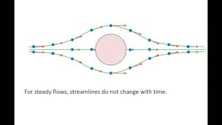
12.2.2. Definitions of the Streamlines

And at the entrance points and the velocity at the exit point will be the 3. And the velocity distributions is given with respect to the x directions this is the about the nozzles.

In fluid dynamics, when we discuss flows, we focus on how velocity changes from one point to another. Here, at the entrance point of a nozzle, we consider the velocity and how it changes as fluid flows through the nozzle to the exit point. The velocity distribution graphically shows how speed varies along the flow direction (in this case, the x-direction). Understanding this transition is crucial because it can affect the overall performance and efficiency of the system.

Imagine a garden hose. When you place your thumb over the end, the area narrows and the water speeds up as it exits; this is similar to how velocity increases at the exit of a nozzle due to a decrease in cross-sectional area.

What we have to need to compute it? What is the acceleration in the x directions? du/dt at the entrance point at this x = 0 that is what the entrance and this is what of exit of the flow.

In this section, we are interested in calculating how the velocity of the fluid changes over time, specifically in the horizontal (x) direction. This change in velocity over time is termed 'acceleration' and is denoted as du/dt. To determine this, we need to evaluate the velocity at the entrance point (x = 0) and at the exit point of the nozzle, where the flow velocity reaches its maximum value.

Continuing with the garden hose analogy, as you adjust your thumb, the speed of the water changes. If you measure how much faster the water becomes as you slowly cover the end, you're essentially measuring acceleration, similar to how we calculate du/dt in fluid flow.

As given in the figure also I am just highlighting it this is the what 1 dimensional flow only x directions component what we have. That means the by definitions the accelerations and along the x directions accelerations the accelerations in the x directions can be written as very simple forms.

In a one-dimensional flow, we simplify our calculations because we only need to consider changes along a single axis (the x-axis). Under these conditions, we can express acceleration in straightforward mathematical terms. By using the derivative of the velocity, we can show how acceleration is related to changes in velocity along that single dimension. This simplification helps in solving complex flow dynamics more efficiently.

Think of a car driving down a straight road. You can easily calculate how its speed (velocity) changes as it accelerates. Since it moves only forward or backward (one dimension), the calculations are simpler than if the car were moving around curves or changes directions constantly.

What are the components can be neglected as it is a steady flow there is no time component on this.

In steady flow, the fluid's properties at a point do not change over time. This means that while we can measure velocities and accelerations, the time component you would normally consider becomes negligible. In practice, this allows us to ignore certain complex variables that might otherwise complicate our calculations, focusing instead on the spatial changes in velocity.

Imagine a calm lake. If someone throws a stone into it, the ripples spread out steadily and don’t change over time in any one location—the surface remains steady over time, similar to our steady flow condition.

If you just substitute this value and do a partial derivative of this u with respect to x and if you substitute it will get it the du that by substitute it is ...

To find specific values for acceleration, we take our velocity function and apply the mathematical technique of partial differentiation with respect to the x-axis. This allows us to isolate changes due to the position in the flow field, leading to a clear calculation of how acceleration varies at different points along the nozzle.

Imagine a graph where you plot the speed of a car as it moves down a straight road. By looking at the graph at different points, you can determine how fast the car is speeding up or slowing down at each moment, similar to how we use partial differentiation to find accelerations at specific points in the flow.

We will get it du/dt = 600 feet per second square which is given is 3 times of V0.

At the exit point of the nozzle, the acceleration computed reveals how much the velocity has increased compared to the entrance point. The calculation shows that at this point, the acceleration is significantly higher (3 times the initial velocity), illustrating how effective the nozzle design is in increasing flow speeds—a critical consideration in nozzle engineering.

Consider a slide in a water park. When you first push off from the top, you're at a slower speed, but as you go down the slide, gravity accelerates you, and by the time you reach the bottom, you're going much faster; this showcases how design can enhance speed.

--