
Steady Flow and Partial Derivatives
Enroll to start learning
You’ve not yet enrolled in this course. Please enroll for free to listen to audio lessons, classroom podcasts and take practice test.
Interactive Audio Lesson
Listen to a student-teacher conversation explaining the topic in a relatable way.
Introduction to Steady Flow
🔒 Unlock Audio Lesson
Sign up and enroll to listen to this audio lesson

Today, we will discuss steady flow in fluids, which is characterized by the velocity at any given point not changing over time.

What do we mean by steady flow? Does that mean the speed is constant?
Not exactly. Steady flow means that, at any point in the fluid, the flow velocity is consistent over time — it does not vary. However, different points may still have different velocities.

So, if I have a nozzle that's narrowing, the fluid speed will increase, right?
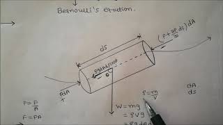
Correct! This leads us to the Bernoulli principle, which indicates that as the flow area decreases, the flow speed increases.

How do we calculate the acceleration under these conditions?
Great question! We'll use partial derivatives to derive the acceleration in the x-direction, and give you a chance to see how the equations work in an actual example.

Can we see some equations now?
Absolutely! Let’s explore some equations relating to velocity distributions.
Velocity Distributions
🔒 Unlock Audio Lesson
Sign up and enroll to listen to this audio lesson

The velocity distribution for fluid flow through a nozzle can greatly affect the outcome of various calculations.
How do we graphically represent these distributions?
Velocity distributions can be represented as functions of position, often utilizing variables such as x to show how velocity changes at different points.
What’s a common equation we might use?
A typical equation is u(x), which can be derived from the principles we've discussed prior.
I see! So using that, we also compute acceleration, right?
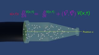
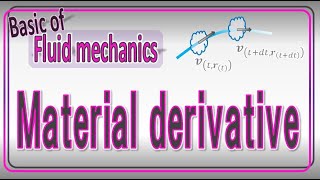
Exactly! The acceleration can be derived from the total time derivative, and then further broken into partial derivatives for local and convective components.
Can you repeat that 'total derivative' part?
Certainly! The total derivative includes changes over both time and space. For steady flow, we interpret some derivatives as zero.
Calculating Accelerations
🔒 Unlock Audio Lesson
Sign up and enroll to listen to this audio lesson
Now that we have velocity definitions, let’s calculate accelerations in the x-direction.
I remember that we need to use u and some variables; how do we start?
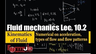
Using the known velocities at the entrance and exit points of our flow, we can apply the partial derivative of our velocity function to find acceleration.
What values would you substitute?
We’ll substitute known values for velocity like V at different points along with the nozzle’s length.
Is this where we find those accelerations at x=0 and x=L?
Exactly! By substituting x values, we derive the accelerations at both the entrance and exit points.
Can we practice that together now?
Yes! Let’s work through an example on the board.
Examples and Problems
🔒 Unlock Audio Lesson
Sign up and enroll to listen to this audio lesson
Let’s look at a specific problem regarding the accelerated flow through a converging nozzle.
What kind of values will be given in typical problems?
You might have velocities, lengths, and sometimes pressures at different points.
Are we looking for changes in velocity over space?
That's right! And we need to apply our derivative concepts to relate these values.
Can we summarize how we solve?
First, we define velocities, use given data to calculate derivatives, and assemble everything for our final acceleration calculations.
It sounds manageable! Let’s practice a sample question.
Absolutely! Practice makes perfect. Let’s tackle one now!
Introduction & Overview
Read summaries of the section's main ideas at different levels of detail.
Quick Overview
Standard
In this section, we explore how steady flow conditions in fluids can be characterized through partial derivatives. By analyzing velocity distributions and acceleration components, we can gain insights into flow behaviors at various points, specifically at the entrance and exit of nozzles. The mathematical underpinnings illustrate how to compute these accelerations under one-dimensional flow assumptions.
Detailed
The section elaborates on the computations involved in understanding steady flow in fluid dynamics, particularly how to derive velocity distributions and the acceleration components. It begins by defining the concept of steady flow and applying it to the situation of converging nozzles, where the velocity increases as the cross-section decreases. The equations presented allow us to compute the x-direction component of acceleration, highlighting the role of partial derivatives in steady flow conditions. Notably, since we are dealing with a steady flow where time factors can be neglected, it simplifies the acceleration equations significantly. The section provides examples and problems that solidify the understanding of how to compute the dynamics of steady flows mathematically, ultimately emphasizing the importance of partial derivatives in analyzing fluid motion.
Youtube Videos


Audio Book
Dive deep into the subject with an immersive audiobook experience.
Velocity Distributions in Nozzles
Chapter 1 of 5
🔒 Unlock Audio Chapter
Sign up and enroll to access the full audio experience
Chapter Content
And at the entrance points and the velocity at the exit point will be the 3. And the velocity distributions is given with respect to the x directions this is the about the nozzles. The velocity field is given as the 2u√(2pat)/p1. This is what the velocity distributions given to us.
Detailed Explanation
In this chunk, we begin by discussing the velocity distributions relevant to flow through nozzles, which shows how velocity varies along the x-axis. The mention of entrance and exit points indicates that the velocity changes as fluid moves through a nozzle, impacting how fluids behave in different scenarios.
Examples & Analogies
Consider a garden hose. When you cover part of the hose with your finger, the water speeds up and shoots out faster through the narrower opening. This is similar to how velocity increases in a nozzle due to its shape.
Understanding Acceleration in the Flow
Chapter 2 of 5
🔒 Unlock Audio Chapter
Sign up and enroll to access the full audio experience
Chapter Content
What we have to need to compute it? What is the acceleration in the x directions? du/dt at the entrance point at this x = 0 that is what the entrance and this is what of exit of the flow. If it is the conditions we need to compute it what will be the accelerations ax du/dt.
Detailed Explanation
This chunk emphasizes calculating the acceleration of the fluid in the x direction, represented as du/dt. This calculation is essential for understanding how fluid velocity changes over time at given points of the flow, namely at the entrance and exit of the nozzle.
Examples & Analogies
Imagine driving a car. When you press the gas pedal, the car accelerates in the direction it's pointing. In fluid dynamics, we measure acceleration in terms of how quickly the fluid velocity changes at different points as it flows through a nozzle.
Mathematical Formulation of Acceleration
Chapter 3 of 5
🔒 Unlock Audio Chapter
Sign up and enroll to access the full audio experience
Chapter Content
the accelerations in the x directions can be written as very simple forms just taking the definitions that the accelerations will be total derivative of du/dt...local accelerations component and convective acceleration component in the x directions that what were look into it.
Detailed Explanation
In this chunk, we explore how to express acceleration mathematically. Acceleration can be decomposed into local acceleration (change in velocity at a point with time) and convective acceleration (change in velocity due to the movement of fluid particles). This conceptual division helps clarify how fluid velocity can change.
Examples & Analogies
Think of a river. As water flows downstream, it can speed up at certain points (local acceleration) because it is flowing faster at those locations, and it can change speed overall as it bends or narrows (convective acceleration).
Steady Flow Assumption
Chapter 4 of 5
🔒 Unlock Audio Chapter
Sign up and enroll to access the full audio experience
Chapter Content
there is no time component on this. We can make it this is equal to 0 and since it is a 1-dimensional flow as it is a steady flow when there is no time component in the velocity field...
Detailed Explanation
This part asserts that in a steady flow, the properties at any point do not change over time, which simplifies calculations significantly. When assuming a steady flow in one dimension, we can effectively treat many time-dependent terms as zero, allowing for streamlined analysis.
Examples & Analogies
Imagine holding a hose steady in one position - the water flows consistently without changing pressure or speed over time, reflecting a steady flow scenario.
Results of Calculations
Chapter 5 of 5
🔒 Unlock Audio Chapter
Sign up and enroll to access the full audio experience
Chapter Content
We have to find out what will be the velocity when x = 0 and x = L and the V_0 is given to us. So using given data we can compute the accelerations in the x directions du/dt at x = 0...
Detailed Explanation
In this chunk, we apply the previously discussed concepts to compute specific numerical values for acceleration at the entrance and exit points of the nozzle using the formulas derived earlier. These calculations provide critical insights into how velocity profiles change in the flow.
Examples & Analogies
When measuring how fast a car accelerates from a stop (x=0) to a cruising speed (x=L), you can calculate exactly how the speed changes, similar to how we calculate acceleration in a fluid flow scenario.
Key Concepts
-
Steady Flow: This occurs when the velocity at any point in the fluid does not change over time.
-
Partial Derivatives: Used to analyze how a function (e.g., velocity) varies with respect to a single variable.
-
Acceleration Components: Includes local and convective accelerations which contribute to the overall acceleration in fluid flow.
-
Velocity Distribution: Refers to how the flow velocity varies with position in the system.
Examples & Applications
In a converging nozzle, the velocity increases as the cross-sectional area decreases, governed by the continuity equation.
For steady flow conditions, the acceleration can be described using partial derivatives, allowing for simplifications in complex flow situations.
Memory Aids
Interactive tools to help you remember key concepts
Rhymes
In steady flow, you'll always find, Velocity stays constant — keep that in mind!
Stories
Imagine a river where the current flows unchangingly; various spots have different speeds, yet none change overtime — that's steady flow!
Memory Tools
To remember local vs. convective acceleration, imagine 'Local Love' is about change over time while 'Convective Cloud' moves with the flow!
Acronyms
Remember PLAC
Partial derivatives relate to Local Acceleration and Convective acceleration.
Flash Cards
Glossary
- Steady Flow
A type of fluid flow where the velocity at any point does not change with time.
- Partial Derivative
A derivative that represents how a function changes as one of its variables changes while keeping other variables constant.
- Convective Acceleration
Acceleration resulting from the change in velocity due to the spatial change of a fluid parcel's position.
- Local Acceleration
Acceleration due to the change in velocity at a specific point in the flow field with respect to time.
- Velocity Distribution
The variation of the velocity of a fluid at different points in a flow field.
Reference links
Supplementary resources to enhance your learning experience.