
Streamline Patterns and Acceleration Field
Enroll to start learning
You’ve not yet enrolled in this course. Please enroll for free to listen to audio lessons, classroom podcasts and take practice test.
Interactive Audio Lesson
Listen to a student-teacher conversation explaining the topic in a relatable way.
Introduction to Velocity Distributions
🔒 Unlock Audio Lesson
Sign up and enroll to listen to this audio lesson

Today we start with analyzing velocity distributions in nozzle flow. Can anyone explain what we might expect in a converging nozzle?

I think the velocity increases as the nozzle narrows, right?
Exactly! The principle of continuity states that as the area decreases, velocity must increase to maintain mass flow rate. Now, the velocity field can be expressed in the form of a formula. We define the velocity's dependence on position. Can someone help identify the primary variables?

I believe it's mainly the position along the x-axis and sometimes the time.
Good! The variables x and t are indeed crucial since flow can be steady or transient. Let's remember this with the acronym 'VPT', meaning 'Velocity depends on Position and Time'.

That makes it easier to remember!
Great! We will now move on to discuss how we calculate acceleration based on these velocity distributions.
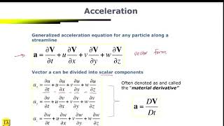
Acceleration Components
🔒 Unlock Audio Lesson
Sign up and enroll to listen to this audio lesson

We need to compute the acceleration components in fluid flow. Can anyone tell me how we approach this mathematically?

Is it by taking the total derivative of the velocity concerning time and space?
Exactly! Our goal is to calculate the local and convective acceleration. For our setup, when we have steady flow, the time derivative can become zero, simplifying our calculations. What does that imply for our equations?
I guess it means we only focus on spatial changes in velocity.
Correct! The acceleration becomes mainly focused on how the velocity changes with respect to x. This leads us to compute specific values at the entrance and exit of our nozzle now.
How do we determine these values mathematically?
By substituting the velocity equations we've established. Each substitution gives us physical insight into the flow, which is pivotal in applications like jet propulsion. Any thoughts on where we might use this in real-world scenarios?
Definitely in aerospace engineering for designing jet engines.
Absolutely! To conclude our session, remember the term 'ACC', for 'Acceleration Calculations depend on the Continuity principle.' Keep this in mind!
Two-Dimensional Flow Patterns
🔒 Unlock Audio Lesson
Sign up and enroll to listen to this audio lesson
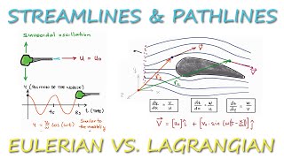
Now, let's explore how we apply these principles in two-dimensional flow. What do we think a streamline is?
A path that a fluid particle follows, right?
Yes! And streamlines help visualize flow and identify acceleration fields. How would we express this mathematically?
We would differentiate the velocity components?
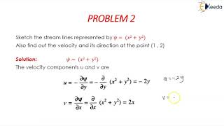
Exactly! We derive the relationships between stream functions and accelerations, which can involve integrating velocity components. What is significant in sketching stream patterns?
I think it shows how fluid moves around objects, like a cylinder.
Right! Sketching these helps to visualize how acceleration can vary. Remember 'FFD' - 'Flow Field Dynamics', to keep these ideas cohesive. Any further questions before we wrap up?
No, I think we've covered a lot!
Great! Always remember the core concepts involving velocity, acceleration, and flow patterns. Thank you for your participation!
Introduction & Overview
Read summaries of the section's main ideas at different levels of detail.
Quick Overview
Standard
The section explores the velocity field in one-dimensional flow through converging nozzles, deriving acceleration components based on velocity variations. It discusses the simplification of the flow parameters, leading to calculations for acceleration at the entrance and exit points of the nozzle.
Detailed
Detailed Summary
This section delves into the fundamental principles of fluid dynamics by analyzing the velocity distributions and acceleration fields associated with certain flow scenarios. Initially, the discussion starts with the characteristics of one-dimensional flow through converging nozzles, emphasizing how velocity variations alter across the nozzle's entry and exit points. Theoretical foundations are laid out through equations to define the velocity field, specifically referencing a derived formula that emphasizes the dependence of velocity on its spatial variable.
The first half of the section focuses on calculating acceleration (both local and convective) based on the changes in velocity with respect to position and time. It explains how to derive the total derivative to understand acceleration better. A critical point noted is that under steady flow conditions and in one-dimensional scenarios, the change in velocity with respect to time can often be neglected, simplifying the calculations. Both the entrance and exit accelerations are evaluated, demonstrating a clear approach to identify how these values correspond to changes in flow characteristics.
Furthermore, the section also provides examples that showcase two-dimensional flow patterns, explaining stream functions and their relation to acceleration fields. By deriving equations for the acceleration in two-dimensional contexts, it builds a compelling case for understanding fluid motion through varying geometries. Lastly, the analysis is rounded off with examples that apply these concepts in practical scenarios like flow around circular cylinders, further enhancing the reader's grasp of fluid dynamics principles.
Youtube Videos


![Components of Acceleration Field [Fluid Mechanics #14]](https://img.youtube.com/vi/G_mG5ALxFrY/mqdefault.jpg)
Audio Book
Dive deep into the subject with an immersive audiobook experience.
Understanding Velocity Distributions in Nozzles
Chapter 1 of 4
🔒 Unlock Audio Chapter
Sign up and enroll to access the full audio experience
Chapter Content
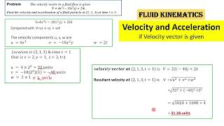
At the entrance point, the velocity at the exit point will be the 3\(V_0\). The velocity distributions are given with respect to the x direction, particularly about the nozzles. The velocity field is presented mathematically.
Detailed Explanation
In fluid dynamics, especially when dealing with nozzles, it's crucial to understand how velocity behaves as fluid enters and exits. The velocity at the entrance of the nozzle is defined as 3 times a reference velocity \(V_0\). This value indicates how the fluid accelerates as it moves through the nozzle, where the cross-sectional area decreases. The provided equations help represent this behavior in a mathematical context, allowing us to compute various parameters related to fluid flow, including acceleration.
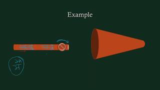
Examples & Analogies
Imagine water flowing through a garden hose. When you partially cover the end of the hose with your thumb, the water accelerates and shoots out faster due to the reduced area. In this example, the entrance point is where the water enters the hose, and the exit point is where it exits out of the nozzle with increased speed.
Computing Acceleration in the x Direction
Chapter 2 of 4
🔒 Unlock Audio Chapter
Sign up and enroll to access the full audio experience
Chapter Content
To compute the accelerations in the x directions \(a_x = \frac{du}{dt}\) at the entrance point at \(x = 0\) and the exit of the flow. If \(V_0 = 10\) feet/second and the length is 1 feet, we need to evaluate the accelerations to understand fluid dynamics in this scenario.
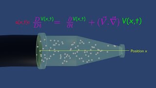
Detailed Explanation
The acceleration of the fluid in the x direction can be derived from the change in velocity over time. This relationship is represented by the equation \(a_x = \frac{du}{dt}\). We substitute our known values, which allows us to calculate the acceleration at two points: the entrance (where \(x = 0\)) and the exit (at maximal velocity). Understanding these accelerations helps predict how the fluid behaves in the nozzle and the forces acting on it.
Examples & Analogies
Think of a car accelerating on a straight road. The speed of the car increases as it moves from a stop at a red light (entrance) to its top speed (exit). The relationship between how quickly the car's speed changes relates directly to the concept of acceleration we discuss in fluid dynamics.
Significance of Steady Flow and 1-Dimensional Flow
Chapter 3 of 4
🔒 Unlock Audio Chapter
Sign up and enroll to access the full audio experience
Chapter Content
In a steady flow scenario, certain components can be neglected. Since there is no time component in this 1-Dimensional flow, several components become 0, simplifying our calculations.
Detailed Explanation
In fluid dynamics, steady flow implies that the fluid's properties at any given point do not change over time. This assumption allows us to disregard time-dependent components, streamlining our calculations. By focusing solely on the spatial dimensions (like the x direction), we can analyze the flow behavior more effectively, making the problem easier to solve mathematically.
Examples & Analogies
Consider a water stream flowing steadily through a pipe. If the water’s speed and pressure are consistent along the pipe, we can simplify our calculations as if nothing changes over time, enabling us to predict outcomes accurately without tracking every moment.
Relationship Between Fluid Velocity and Acceleration
Chapter 4 of 4
🔒 Unlock Audio Chapter
Sign up and enroll to access the full audio experience
Chapter Content
We can compute how acceleration \(a_x\) varies with respect to x and functions in terms of \(V\) and the length \(L\). We find the velocity when \(x = 0\) and \(x = L\), allowing us to determine the acceleration at these points.
Detailed Explanation
The change in acceleration with position provides insight into the fluid dynamics as it acts through the nozzle. By calculating velocities at designated positions (entrance and exit), we can relate those velocities back to accelerations through the equation we previously discussed. Recognizing how these values interplay gives us a clearer picture of the forces at play during fluid motion.
Examples & Analogies
Imagine tracking an athlete's speed on a running track. By noting the athlete's speed at different markers (like the start and end of a sprint), you can calculate acceleration and understand how quickly the athlete speeds up or slows down.
Key Concepts
-
Velocity Field: Represents how velocity varies in fluid flow, especially in confined spaces like nozzles.
-
Acceleration: Divided into local and convective components, which help quantify how speed changes in fluid dynamics contexts.
-
Streamlines: Useful in visualizing flow paths and are essential in analyzing acceleration patterns.
Examples & Applications
The increase in speed as fluid flows through a narrowing nozzle.
Calculation of acceleration at the entrance and exit of a nozzle to understand flow dynamics.
Memory Aids
Interactive tools to help you remember key concepts
Rhymes
As the nozzle tightens, speed will rise; fluid flows fast, as if it flies.
Stories
Imagine a river flowing through a narrow canyon, where the water speeds up as it passes through, demonstrating how nozzles work.
Memory Tools
Use 'ACC' - Acceleration Calculations depend on Continuity to remember how to derive acceleration from velocity changes.
Acronyms
VPT - Velocity depends on Position and Time.
Flash Cards
Glossary
- Velocity
The speed of something in a given direction, often analyzed in fluid dynamics to understand flow characteristics.
- Acceleration
The rate of change of velocity of an object, important in evaluating how velocity changes in fluid flow.
- Streamline
A path traced by a particle in a fluid flow, aiding in visualizing the flow and its patterns.
- Converging nozzle
A nozzle design where the cross-sectional area decreases, typically leading to an increase in fluid velocity.
- Local acceleration
Acceleration due to changes in velocity at a specific point in time.
- Convective acceleration
Acceleration resulting from the movement of fluid particles through a velocity field.
Reference links
Supplementary resources to enhance your learning experience.