
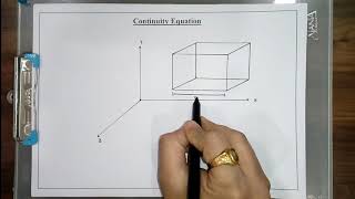
Scalar Components in Cartesian Coordinates
Enroll to start learning
You’ve not yet enrolled in this course. Please enroll for free to listen to audio lessons, classroom podcasts and take practice test.
Interactive Audio Lesson
Listen to a student-teacher conversation explaining the topic in a relatable way.
Introduction to Scalar Components
🔒 Unlock Audio Lesson
Sign up and enroll to listen to this audio lesson

Good morning class! Today, we will focus on the scalar components of velocity in Cartesian coordinates. Can anyone tell me what scalar components represent in fluid mechanics?

Are they the speed of the fluid in each direction, like x, y, and z?
Exactly! We denote them as u, v, and w respectively for the x, y, and z directions. These components are crucial because they tell us how fluid is moving in three-dimensional space.

Why is it important to understand these components?
Understanding these components allows us to derive the Navier-Stokes equations, which govern fluid flow. Remember, it's vital to see how they interact over time and space.

Can these components change over time?
Yes, they can vary with time and position. This is why we express them as functions of time, t, and spatial coordinates, x, y, and z. Great question!

What tools do we use to analyze these changes in real-life scenarios?
We typically use Computational Fluid Dynamics tools like CFD to model these scenarios based on our understanding of scalar components.
To summarize, scalar components u, v, and w are essential for analyzing velocity in fluid mechanics, acting as foundations for deeper equations like the Navier-Stokes.
Deriving from Scalar Components to Navier-Stokes
🔒 Unlock Audio Lesson
Sign up and enroll to listen to this audio lesson

Now that we understand scalar components, let’s discuss how we derive the Navier-Stokes equations from them. Who can explain what Navier-Stokes equations are?
Aren't they equations that describe the motion of fluid substances?
Correct! They describe how fluid moves based on various forces. You will see that these scalar components play a pivotal role in forming these equations.
How do we connect scalar components to the Navier-Stokes equations?
By applying the continuum hypothesis and the differential forms of our scalar components, we can relate them to stress tensors and body forces. This will be seen in our derivations.
What about the assumptions? Do we need them to derive these equations?
Yes, we need assumptions like continuity and differentiability of these scalar fields in space and time, along with applying Taylor's series to approximate changes across control volumes.
Could you summarize the significance of this derivation?
Sure! The derivation connects theoretical concepts of fluid mechanics with practical modeling techniques, underscoring the utility of scalar components in analyzing fluid dynamics.
Applications of Scalar Components in CFD
🔒 Unlock Audio Lesson
Sign up and enroll to listen to this audio lesson
Let’s discuss how these scalar components are practically applied in CFD. Can anyone give an example where scalar velocity components are used?
The flow around a bridge pier?
Exactly! In such scenarios, we can model the velocity field by analyzing how these components change over time and space to predict flow behavior.
What results do we obtain from these models?
We obtain critical information like pressure distributions and how they affect structures, which help engineers design safer and more efficient systems.
Are there limitations to this approach?
Yes, the Navier-Stokes equations do have limitations, particularly under turbulent conditions. But by understanding scalar components, we can address some challenges effectively.
Can we visualize these changes?
Definitely! Visualizing the velocity fields alongside scalar components allows us to see flow patterns that guide decision-making in engineering practice.
In summary, scalar components are not just abstract concepts; they are practical tools in CFD applications that provide essential insights for real-world engineering problems.
Introduction & Overview
Read summaries of the section's main ideas at different levels of detail.
Quick Overview
Standard
Scalar components of velocity in Cartesian coordinates are crucial for understanding fluid mechanics, particularly in the context of Navier-Stokes equations. This section covers the definitions, derivations, and applications involving scalar velocity components, emphasizing the role these concepts play in analyzing fluid flow based on spatial and temporal variables.
Detailed
Scalar Components in Cartesian Coordinates
In fluid mechanics, scalar components of velocity are expressed in Cartesian coordinates as functions of position (x, y, z) and time (t). This section elaborates on various aspects of scalar components in relation to velocity fields and their significance in deriving the Navier-Stokes equations. Scalar components, designated as u, v, and w, represent fluid velocities in the x, y, and z directions, respectively. These scalars capture the essence of how fluid properties behave in space and time, aiding in the computational modeling of fluid systems through tools like computational fluid dynamics (CFD).
Understanding these components is essential for solving complex flow problems, such as the flow around a bridge pier, where how velocity fields and pressure change are modeled mathematically. The section emphasizes applying Taylor series on differential control volumes to derive crucial relationships that illustrate how momentum flux, stress tensors, and body forces manifest in fluid mechanics. These aspects form the foundational aspects to tackle real-world fluid dynamic problems.
Youtube Videos


Audio Book
Dive deep into the subject with an immersive audiobook experience.
Introducing Scalar Components
Chapter 1 of 5
🔒 Unlock Audio Chapter
Sign up and enroll to access the full audio experience
Chapter Content
Here I am looking just Cartesian coordinate systems. In that I have the uvw, so this is small v. the scalar component in x directions of velocity field which is a functions of space and the time.
Detailed Explanation
In fluid mechanics, scalar components refer to quantities that can be described just by a single value per point in space and time. For example, the velocity field can be represented in three dimensions using Cartesian coordinates (x, y, z). The components of velocity are defined as 'u', 'v', and 'w' along the x, y, and z directions respectively. These components are not fixed; instead, they vary depending on both the position in the fluid and the time. This means to fully describe the flow of fluid at any point, we need to know how these scalar components change over space and time.
Examples & Analogies
Imagine standing at a beach and watching the waves. The velocity of water at any point in the ocean is not just one single speed; it can differ based on where you are. If you measure the speed of water at different depths and distances from the shore, you're effectively measuring 'u', 'v', and 'w' at different points, akin to how we describe fluid flow in three-dimensional space.
Functions of Position and Time
Chapter 2 of 5
🔒 Unlock Audio Chapter
Sign up and enroll to access the full audio experience
Chapter Content
That is what I try to introduce in the very beginning classes to say that the scalar components having this functions of positions and the time as it is a Cartesian coordinate systems we are defining as x, y, z and the t the same way if you talk about small v which is the scalar components of in the y directions of velocity components also a functions of x, y, z, t.
Detailed Explanation
In fluid dynamics, when discussing scalar components, it's essential to recognize that these quantities are functions of both position and time. For instance, the scalar component of velocity in the x-direction depends not only on its position in the three-dimensional space defined by 'x', 'y', and 'z', but also changes over time, denoted by 't'. This means that to understand the fluid flow at any specific location and time, we must consider how these quantities interact and vary.
Examples & Analogies
Think of a city's traffic flow. The speed of cars on a road isn't constant and varies not only based on where you are along the road but also at what time of day it is. During rush hour, the speed slows down due to congestion, while at midnight, you may find vehicles speeding. Similarly, in fluid mechanics, these scalar components of velocity change with respect to both their location and time.
Describing Velocity Fields in 3D
Chapter 3 of 5
🔒 Unlock Audio Chapter
Sign up and enroll to access the full audio experience
Chapter Content
These are all these functions we are talking about. and using this computational foot diameter tools for a complex flow like flow around a bridge spire, we are solving it and what we are getting it how the velocity fields are changing, how the pressure fields are changing.
Detailed Explanation
To study fluid behavior, engineers and scientists often use computational tools to model the velocity fields and pressure fields around objects like bridge piers. The velocity field gives the speed and direction of the fluid at every point in a three-dimensional space. Understanding how these velocity and pressure fields change helps in predicting fluid behavior and making engineering decisions.
Examples & Analogies
Consider a leaf floating in a river. The leaf's movement changes as the water flows around a rock. Using computational tools, one can visualize how the water's speed and direction change around that rock. Similarly, in engineering, simulating these scenarios helps ensure that structures like bridges are safe and can withstand forces from flowing water.
Understanding Computational Fluid Dynamics
Chapter 4 of 5
🔒 Unlock Audio Chapter
Sign up and enroll to access the full audio experience
Chapter Content
When you have that problems, here we have considered a problems with a bridge pier. And here if you look at how the velocity field changes with the velocity field which has a component of scalar component and in three directions.
Detailed Explanation
Computational Fluid Dynamics (CFD) is a tool used to solve fluid flow problems, such as understanding how water moves around a bridge pier. By breaking the flow down into scalar components in three-dimensional Cartesian coordinates, engineers can gain insights into how water flows in different directions and under varying conditions.
Examples & Analogies
Think of a water hose spraying water. The spray pattern is affected by how the water moves in different directions depending on the angle of the hose. In CFD, we analyze how the fluid's behavior changes around obstacles like a bridge pier, allowing for better design and safety assessments in scenarios like extreme weather events.
Importance of Understanding Velocity Fields
Chapter 5 of 5
🔒 Unlock Audio Chapter
Sign up and enroll to access the full audio experience
Chapter Content
Now if I go for the next ones if you look it how do we get this computational fluid dimension solutions by solving these equations okay solving these equations which is known as very famous is Navier-Stokes equations.
Detailed Explanation
The Navier-Stokes equations are fundamental in fluid mechanics for describing how fluids flow. These equations incorporate the principles of conservation of mass, momentum, and energy, allowing scientists and engineers to model complex fluid dynamics accurately. The solutions to these equations help in understanding the motion of fluid particles throughout a system, which is crucial for designing various engineering applications.
Examples & Analogies
Consider how weather models predict wind patterns and storms. The equations behind these models, including the Navier-Stokes equations, are complex but essential for accurate forecasting. In the same way, when analyzing water flows around structures or during environmental studies, these equations play a pivotal role in understanding and predicting flow behavior.
Key Concepts
-
Scalar Components: Represent fluid motion in specific directions (u, v, w) and crucial for understanding flow dynamics.
-
Navier-Stokes Equations: Govern fluid motion by correlating various forces acting on the fluid.
-
Computational Fluid Dynamics (CFD): A numerical approach to simulate fluid flow, relying on concepts of scalar components.
Examples & Applications
Using scalar components to analyze the velocity field in a river's flow.
Modeling the pressure distribution around structures like bridge piers using CFD based on scalar components.
Memory Aids
Interactive tools to help you remember key concepts
Rhymes
U for X and V for Y, W’s the Z where fluids flow high.
Stories
Imagine a river splitting into three branches: one flows towards the mountain peak (u), another through lush valleys (v), and the last into the depths of the ocean (w). Each shows fluid movement in specific paths.
Memory Tools
UVW - Understand the Velocity's Way in three dimensions!
Acronyms
C-F-D for Computational Fluid Dynamics - the Field of Fluid Analysis!
Flash Cards
Glossary
- Scalar Components
Components that represent movement in a specific direction within fluid dynamics, denoted as u (x-direction), v (y-direction), and w (z-direction).
- NavierStokes Equations
A set of equations that describe the motion of fluid substances, detailing how forces affect fluid motion over time.
- Computational Fluid Dynamics (CFD)
A computational tool used to simulate fluid flow and analyze the physical properties of fluids using numerical analysis.
- Continuum Hypothesis
An assumption in fluid mechanics that a fluid is continuous, allowing for the application of differential calculus to fluid properties.
- Taylor Series
A representation of a function as an infinite sum of terms calculated from the values of its derivatives at a single point.
Reference links
Supplementary resources to enhance your learning experience.