
Op-Amp-based Integral Control Circuits
Interactive Audio Lesson
Listen to a student-teacher conversation explaining the topic in a relatable way.
Introduction to Integral Control Circuits
🔒 Unlock Audio Lesson
Sign up and enroll to listen to this audio lesson

Today, we will discuss integral control circuits that utilize Op-Amps to address steady-state errors. Can anyone tell me why it's important to eliminate these errors?

Is it to ensure that the system reaches the desired output without lingering fluctuations?
Exactly! Integral control helps us achieve that by integrating the error over time, thus providing a corrective response. This leads us to how we design these circuits.

How is the output of an integral control circuit calculated?
Great question! The output voltage is given by the equation Vout(t) = (1/RC) ∫ E(t) dt. Here, R and C define the characteristics of the integrator.
Remember the acronym 'ICE' - Integral for eliminating errors. This will help you recall the role of integral control!

What kind of applications are suited for integral control?
Integral control circuits are fantastic for precision systems, like those ensuring a mechanical system stays at a set position. Let’s summarize: they are critical for stability and error correction!
Lab Work and Construction
🔒 Unlock Audio Lesson
Sign up and enroll to listen to this audio lesson

Now, let’s transition to the lab work! Who can remind us of the materials we need to build an integral control circuit?

We need an Op-Amp, resistors, capacitors, and a signal generator!
Correct! The Op-Amp will function as the integrator, while resistors and capacitors will set our integration time. What do you think we'll observe when we apply an error signal?
I suppose the output will change based on the accumulated error over time.
Yes! And thus, we'll measure how effectively the circuit can correct for steady-state errors. Always remember that practical experience solidifies theoretical concepts. Let's summarize: understanding the design basics is critical for successful implementation!
Applications and Real-life Context
🔒 Unlock Audio Lesson
Sign up and enroll to listen to this audio lesson
Finally, let's explore where integral control circuits are applied. Why might industries rely on these circuits?
They might use them in temperature control systems to maintain set temperatures.
Absolutely! They keep systems stable, eliminating small errors over time. Can you think of other examples?
Position control in robotics could definitely use integral control to ensure accuracy.
Excellent points! So remember, integral control circuits play a pivotal role in ensuring precision across many applications. Let’s summarize our key points before we wrap up.
Introduction & Overview
Read summaries of the section's main ideas at different levels of detail.
Quick Overview
Standard
Integral control circuits utilize operational amplifiers (Op-Amps) to produce an output proportional to the accumulated error over time, effectively eliminating steady-state errors. This section covers the design principles, key equations, applications, and lab work involved in constructing these integral control circuits.
Detailed
Overview of Integral Control Circuits
Integral control circuits play a vital role in control systems, particularly when eliminating steady-state errors is critical. By utilizing operational amplifiers (Op-Amps) in an integrator configuration, these circuits integrate the error signal over time, producing an output that reflects the cumulative error.
Key Features and Design
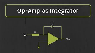
- Basic Design: The Op-Amp is configured to integrate the error signal, creating an output that increases or decreases based on the cumulative error. This design is fundamental in achieving accurate control in various automation scenarios.
- Key Equation: The output voltage (
V_{out}(t)
) is given by:
V_{out}(t)= rac{1}{RC} orall E(t) dt
where R and C are the resistor and capacitor values that determine the time constant of the integrator.
- Applications: Integral control is particularly useful in precision applications and position control, ensuring the system reaches and maintains a desired setpoint without steady-state errors.
Lab Work
The practical implementation involves constructing an integral control circuit using Op-Amps, resistors, and capacitors, where students will apply an error signal and observe how the output responds to accumulated error over time. This hands-on approach solidifies theoretical concepts with practical experience.
Youtube Videos
Audio Book
Dive deep into the subject with an immersive audiobook experience.
Introduction to Integral Control Systems
Chapter 1 of 5
🔒 Unlock Audio Chapter
Sign up and enroll to access the full audio experience
Chapter Content
In an integral control system, the control output is proportional to the accumulated sum (or integral) of the error signal over time. Integral control is used to eliminate steady-state errors and ensure that the system reaches the desired setpoint.
Detailed Explanation
Integral control focuses on how much error has accumulated over time. When there is a difference between the desired output (setpoint) and the actual output, integral control continuously adds up this error. By accumulating this value, integral control can adjust the system output to eliminate persistent errors that would prevent the system from reaching the setpoint. Essentially, if a system is consistently underperforming or overperforming, integral control helps to correct this over time.
Examples & Analogies
Think of a water tank that is supposed to be filled with water to a certain level (the setpoint). If the water level is consistently low (the error), an integral controller would keep adding water to compensate for the slow filling over time. Gradually, it works to bring the water level up to the desired point. If only using proportional control, you might never fully fill the tank because it only reacts to the immediate difference between the current level and the setpoint.
Design of Integral Control Circuits
Chapter 2 of 5
🔒 Unlock Audio Chapter
Sign up and enroll to access the full audio experience
Chapter Content
● Basic Design:
○ The Op-Amp is configured in an integrator configuration, where the error signal is integrated over time to produce an output that increases or decreases based on the accumulated error.
Detailed Explanation
To design an integral control circuit, the operational amplifier is set up in what’s called an integrator configuration. This involves connecting a resistor (R) and a capacitor (C) in a feedback loop with the Op-Amp. The Op-Amp takes the incoming error signal and integrates it over time, which means it sums up the error continually. As a result, the output voltage reflects the total accumulated error. When the error signal is positive, the output increases, indicating that action needs to be taken to reduce this error.
Examples & Analogies
Imagine a person keeping track of how many hours they’re underperforming at work. Each week, they jot down the number of hours they should have worked versus the number of hours they actually worked. Over time, they have a record of hours lost due to inefficiency (the accumulated error), which they can address to improve future performance. The integral control functions similarly, keeping track of past errors to adjust current performance.
Key Equation for Integral Control
Chapter 3 of 5
🔒 Unlock Audio Chapter
Sign up and enroll to access the full audio experience
Chapter Content
● Key Equation:
○ The control output is given by:
Vout(t)=1RC∫E(t) dt
Where:
■ Vout(t) is the control output,
■ R and C are the resistor and capacitor in the feedback loop,
■ E(t) is the error signal.
Detailed Explanation
The equation for the control output in an integral control circuit helps us understand how the integral of the error signal influences the output. The term 'Vout(t)' refers to the voltage output of the Op-Amp, which tells us how the system adjusts in response to the accumulated error. '1/(RC)' is a scaling factor determined by the resistor and capacitor values, which affects how quickly the system responds. The integral of 'E(t)' over time essentially measures the total error up to the current moment, guiding the necessary adjustments.
Examples & Analogies
In our water tank analogy, the 'integral' part can be likened to keeping a running total of how many liters of water are needed to reach the target level. The resistor and capacitor work together to define how fast the water (or corrective output) is added. If you have a big capacitor, it takes longer to fill the tank fully, much like how a slow and steady approach can ensure the tank doesn't overflow.
Applications of Integral Control
Chapter 4 of 5
🔒 Unlock Audio Chapter
Sign up and enroll to access the full audio experience
Chapter Content
● Applications:
○ Precision systems: Used in systems where the goal is to eliminate steady-state errors.
○ Position control: Ensures that a mechanical system reaches and stays at a set position by accumulating error over time.
Detailed Explanation
Integral control is crucial in applications where precision is vital, such as in robotics, where maintaining a specific position over time is necessary. By ensuring that even small errors are corrected over time, integral control helps achieve a steady-state output without oscillations or persistent errors. For example, a robotic arm needs to reach a designated position and maintain it, where even a minor deviation should be corrected steadily. Integral control systematically addresses any discrepancies.
Examples & Analogies
Consider a robotic vacuum cleaner. If it has an integral control system, it will gradually learn that it has missed a spot over repeated cleaning sessions. It accumulates this 'missed error' and adjusts its cleaning path to ensure it cleans every part of the area effectively over time, correcting past mistakes and improving future cleaning cycles.
Lab Work on Integral Control Circuits
Chapter 5 of 5
🔒 Unlock Audio Chapter
Sign up and enroll to access the full audio experience
Chapter Content
● Objective: Design and build an integral control circuit to regulate the system based on the accumulated error signal.
● Materials:
1. Op-Amp (e.g., LM741)
2. Resistors and capacitors for integration
3. Signal generator and oscilloscope
4. Test system or motor
● Procedure:
1. Construct the integral control circuit and apply an error signal.
2. Observe the output response over time as the error signal is integrated.
3. Measure how the system corrects steady-state errors.
Detailed Explanation
The lab exercise allows students to apply theoretical concepts in a practical environment. By building the integral control circuit with an Op-Amp, students will see firsthand how the circuit responds to applied error signals. Using materials like resistors and capacitors, they can set up the integrator and feed error signals to observe how the accumulated error influences the output response. This hands-on experience solidifies their understanding of the principles of integral control.
Examples & Analogies
This practical exercise is similar to a cooking experiment where you modify a recipe. Just like you might adjust the seasoning over time based on taste (the error signal), in the lab, students adjust the components and observe how it affects the system’s output. Through trial and error, they learn what works best to achieve the ideal control system, reinforcing the concepts of integral control in action.
Key Concepts
-
Integral Control: A method used to eliminate steady-state errors by integrating the error over time.
-
Op-Amp Integration: The use of operational amplifiers in creating integrator circuits.
-
Applications of Integral Control: Precision systems, position control, and more.
Examples & Applications
Using integral control in a temperature control system to ensure the temperature stabilizes at a desired setpoint.
Employing integral control to adjust the position of robotic arms, ensuring they reach and maintain accuracy.
Memory Aids
Interactive tools to help you remember key concepts
Rhymes
Integrate the error well, to bring the output to a stable level.
Stories
Imagine a boat that needs to reach a dock. It adjusts its steering based on how far it's drifted over time, much like how integral control adjusts based on accumulated error.
Memory Tools
ICE stands for Integral Control Eliminates errors - your key to recalling integral control benefits.
Acronyms
IRE stands for Integral, Regulate, Eliminate errors - a handy guide for your studies!
Flash Cards
Glossary
- Integral Control
A control method that accumulates the error over time to minimize steady-state errors.
- OpAmp
An operational amplifier, a type of electronic amplifier used in various configurations.
- Integrator Configuration
The setup of an Op-Amp circuit designed to integrate input signals with respect to time.
- Error Signal
The difference between the desired setpoint and the actual output.
- SteadyState Error
The difference that persists between the desired output and the actual output of a system.
Reference links
Supplementary resources to enhance your learning experience.