
Inner Product Spaces
Enroll to start learning
You’ve not yet enrolled in this course. Please enroll for free to listen to audio lessons, classroom podcasts and take practice test.
Interactive Audio Lesson
Listen to a student-teacher conversation explaining the topic in a relatable way.
Definition of Inner Product Space
🔒 Unlock Audio Lesson
Sign up and enroll to listen to this audio lesson

Welcome everyone! Today, we're diving into inner product spaces. To start, can anyone tell me what defines an inner product space?

Is it related to vectors and how we can measure them?
Absolutely! An inner product space is a vector space equipped with an inner product. This inner product allows us to define lengths and angles. It has three key properties: linearity in the first argument, conjugate symmetry, and positive-definiteness. Does anyone remember what these terms mean?

Linearity means we can distribute scalar multiplication and addition, right?
Correct! Great job, Student_2. And conjugate symmetry refers to the fact that the inner product of two vectors is the same, even if you switch them around. Now, why is positive-definiteness important?

It ensures that the inner product is zero only if the vector is the zero vector, right?
Exactly! Let’s remember that with the acronym LCP for Linearity, Conjugate symmetry, and Positive-definiteness. It summarizes the crucial characteristics of inner product spaces.
To summarize, inner product spaces allow for measuring angles and lengths with their properties guiding the analysis of geometric configurations.
Examples of Inner Product Spaces
🔒 Unlock Audio Lesson
Sign up and enroll to listen to this audio lesson

Now that we understand the definition, let’s look at some examples. Can anyone give me an example of an inner product space?

Euclidean space Rn?
Great! In Euclidean space Rn, the inner product is simply the dot product. It’s defined as the sum of the products of corresponding components. Can someone write out the formula for the inner product of two vectors u and v in Rn?
Sure! ⟨u,v⟩ = u1v1 + u2v2 + ... + unvn.
Nicely done! Now, what about function spaces? What example can we find there?
The space of continuous functions on an interval can have an inner product defined by integration!
Exactly right! The inner product is defined by integrating the product of two functions over a given interval. This is incredibly useful in applications like Fourier series. Remember, understanding these examples can help us see their real-world implications!
Orthogonality and Projection
🔒 Unlock Audio Lesson
Sign up and enroll to listen to this audio lesson
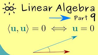
Let's talk about orthogonality now. Who can define orthogonal vectors?
Vectors are orthogonal if their inner product is zero, right?
Exactly right! Orthogonal vectors are at right angles to each other in the geometric sense. Now, can someone explain orthonormal sets?
An orthonormal set consists of orthogonal vectors that are also unit vectors.
Perfect! Now, understanding these concepts is vital for projections. The projection of vector u onto vector v gives us the closest point in the space spanned by v. Does anyone remember the formula for the projection?
Yes! proj_v(u) = (⟨u,v⟩ / ⟨v,v⟩) * v.
Exactly! This projection is vital in many engineering applications, such as least squares approximation. Let’s wrap up here — orthogonality simplifies many solutions in our engineering problems.
Introduction & Overview
Read summaries of the section's main ideas at different levels of detail.
Quick Overview
Standard
Inner Product Spaces extend the concept of dot products to abstract vector spaces, allowing for the definition of lengths and angles in higher dimensions. This section explores the properties, examples, and applications of inner product spaces, particularly their significance in Civil Engineering and numerical methods.
Detailed
Inner Product Spaces
Inner product spaces are a fundamental concept in linear algebra that generalizes the familiar dot product from Euclidean spaces to more abstract vector spaces. This framework allows us to measure angles and lengths, facilitating various applications across geometry, analysis, and engineering disciplines.
Key Points:
- Definition: A vector space is termed an inner product space when it has an additional operation, the inner product, satisfying properties like linearity, conjugate symmetry, and positive-definiteness.
- Examples: Standard inner product spaces include:
- Euclidean spaces
- Complex spaces
- Function spaces such as continuous functions over an interval.
- Orthogonality: The concepts of orthogonal and orthonormal vectors are crucial in simplifying problems, especially through orthogonal decomposition and projections.
- Significance: Inner products underpin methods in structural analysis, finite element analysis, elasticity theory, and least squares approximation. Additionally, the Cauchy–Schwarz inequality and triangle inequality are fundamental results that arise from the inner product structure.
This section is vital for understanding advanced mathematical methodologies that impact engineering and physical sciences.
Youtube Videos


Audio Book
Dive deep into the subject with an immersive audiobook experience.
Definition of Inner Product Space
Chapter 1 of 18
🔒 Unlock Audio Chapter
Sign up and enroll to access the full audio experience
Chapter Content
A vector space V over the field R or C is called an inner product space if it is equipped with an additional operation called the inner product.
Inner Product:
An inner product on a vector space V is a function:
⟨·,·⟩:V ×V →R or C
that satisfies the following properties for all u,v,w ∈ V, and scalar α ∈ R (or C):
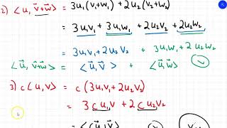
1. Linearity in the First Argument:
⟨αu+v,w⟩=α⟨u,w⟩+⟨v,w⟩
2. Conjugate Symmetry:
⟨u,v⟩=⟨v,u⟩ (For real inner product spaces, this becomes ⟨u,v⟩=⟨v,u⟩)
3. Positive-Definiteness:
⟨v,v⟩≥0, and ⟨v,v⟩=0⇔v =0
Detailed Explanation
An inner product space is a special type of vector space that comes with a function called the inner product, which allows us to measure angles and lengths between vectors. The inner product, represented by ⟨u, v⟩, has three core properties:
1. Linearity: If you scale a vector or add two vectors, the inner product behaves predictably. This means you can factor out scalars and separate components of the inner product.
2. Conjugate Symmetry: The order in which you take the inner product of two vectors doesn't change the result, which is crucial when dealing with complex numbers.
3. Positive-Definiteness: The inner product of a vector with itself is always zero or positive, and it's only zero when the vector itself is the zero vector. This property ensures that we can measure the 'length' of vectors in a meaningful way.
Examples & Analogies
Think of an inner product space like a measuring tape in geometry. Just as a tape measure can help us find distances between points by measuring straight lines and angles, the inner product allows us to measure relationships between vectors. For instance, consider two people stretching a rope between themselves – the angle and length of that rope represent the inner product, helping us visualize geometric relationships.
Examples of Inner Product Spaces
Chapter 2 of 18
🔒 Unlock Audio Chapter
Sign up and enroll to access the full audio experience
Chapter Content
- Euclidean Space Rn
Let u=(u1,u2,...,un) and v =(v1,v2,...,vn), then:
⟨u,v⟩= Σ (u_i * v_i) for i from 1 to n. This is the standard dot product. - Complex Space Cn
Let u,v ∈Cn, then:
⟨u,v⟩= Σ (u_i * v_i) - Function Space
Let V be the space of real-valued continuous functions on the interval [a,b], i.e., V =C[a,b]. The inner product is defined as:
⟨f,g⟩= ∫ from a to b f(x) * g(x) dx
Detailed Explanation
This chunk provides three distinct examples of inner product spaces:
1. Euclidean Space Rn: This is the most familiar inner product space, where the inner product between two vectors u and v is simply their dot product. It calculates the sum of the products of their corresponding entries and reflects the geometric concept of angle and length.
2. Complex Space Cn: In spaces where vectors have complex entries, the inner product involves a summation similar to the Euclidean case, but it includes the complex conjugate to ensure certain properties hold, like positive definiteness.
3. Function Space: This example illustrates that inner products aren't limited to finite-dimensional spaces. In the space of real-valued continuous functions defined on an interval, the inner product is defined by an integral, allowing us to evaluate functions in a manner akin to calculating areas under curves. This is vital in applications like Fourier series.
Examples & Analogies
Imagine you’re measuring the performance of different athletes (the vectors) on a track. For the Euclidean case, you might measure their speeds and calculate an average performance (the dot product). In the complex case, you could be analyzing their performance in a sport that combines multiple elements (like swimming combines speed and technique), and thus you account for additional factors through complex numbers. For functions, think of analyzing different melodies in music; their inner product (integral of the product of the notes) helps you understand how harmoniously they can be combined.
Norm Induced by Inner Product
Chapter 3 of 18
🔒 Unlock Audio Chapter
Sign up and enroll to access the full audio experience
Chapter Content
In an inner product space, the norm or length of a vector v is given by:
∥v ∥= √⟨v,v⟩.
This norm allows us to define distance and angle between vectors.
Detailed Explanation
In any inner product space, the norm of a vector v provides a way to measure its length, calculated as the square root of the inner product of the vector with itself. This norm is critical because it leads us to concepts of distance and angles between vectors. When two vectors are involved, you can determine how far apart the two vectors are based on their norms and their inner product, which gives rise to the cosine of the angle between them.
Examples & Analogies
Think about measuring the height of a tree by using a measuring tape (the inner product) to lay out the height on the ground. You can square the height to get a notion of area under the tree’s shadow and then take the square root to find a linear representation of how 'tall' the tree stands. Similarly, in the inner product space, finding the norm of a vector tells you how long that vector is, just like knowing how tall a tree is informs you about its stature in nature.
Orthogonality and Orthonormality
Chapter 4 of 18
🔒 Unlock Audio Chapter
Sign up and enroll to access the full audio experience
Chapter Content
Orthogonal Vectors:
Two vectors u and v are said to be orthogonal if:
⟨u,v⟩=0.
Orthonormal Set:
A set of vectors {v1,v2,...,vn} is called orthonormal if:
1. ⟨vi,vj⟩=0 for i≠j
2. ∥vi∥=1 for all i.
Orthonormal sets are important in simplifying many problems in engineering, especially when projecting vectors or solving systems using orthogonal decomposition.
Detailed Explanation
Orthogonality is a fundamental concept whereby two vectors are considered orthogonal if their inner product equals zero, akin to perpendicular vectors in geometry. In a broader sense, a set of vectors is orthonormal if not only are they orthogonal to each other, but each vector also has a unit length (norm equals one). Orthonormal sets simplify many calculations in engineering and mathematics, especially when working on projections and decompositions, since these properties allow for clear separations of components.
Examples & Analogies
Imagine you are designing a floor plan for a building. The walls (vectors) should be orthogonal (perpendicular) to each other for practical layout purposes. If one wall is at a right angle to another (orthogonal) and also measures exactly the same height (unit length), you can efficiently plan out rooms with clear dimensions. This is analogous to using orthonormal sets in calculations where you want each measurement to be precise and independent.
The Cauchy–Schwarz Inequality
Chapter 5 of 18
🔒 Unlock Audio Chapter
Sign up and enroll to access the full audio experience
Chapter Content
For any vectors u,v ∈V:
|⟨u,v⟩|≤∥u∥·∥v ∥.
Equality holds if and only if u and v are linearly dependent.
Detailed Explanation
The Cauchy–Schwarz Inequality is a fundamental principle that states the absolute value of the inner product of two vectors cannot exceed the product of their norms. This inequality captures a key relationship between vectors, indicating how their angles and lengths interact. Equality in this case holds only when one vector can be expressed as a scalar multiple of the other, meaning they're in the same direction or are collinear.
Examples & Analogies
Consider two people throwing a ball in a game of catch. The distance they can effectively cover (the limits of their throws) defines how close they can stand to each other while still being able to catch the ball. The Cauchy–Schwarz Inequality translates this concept mathematically, indicating the maximum distance (the product of their 'throwing strengths,' or norms) cannot be exceeded, ensuring that if their throws are direct (linearly dependent), they can catch the ball regardless of distance.
Triangle Inequality
Chapter 6 of 18
🔒 Unlock Audio Chapter
Sign up and enroll to access the full audio experience
Chapter Content
∥u+v ∥≤∥u∥+∥v ∥.
This is a direct consequence of the inner product structure and has important implications in convergence, stability, and bounding solutions.
Detailed Explanation
The Triangle Inequality states that the length of the resultant vector formed by adding two vectors cannot exceed the sum of the lengths of the individual vectors. This geometrical interpretation mirrors the classical triangle inequality in geometry and demonstrates how distances interact in vector spaces. It plays an essential role in analyzing the stability of solutions and convergence during computations.
Examples & Analogies
When you're traveling from one city to another by road, the direct route (vector sum of distances) shouldn't be shorter than simply adding up the distances of each stretch (individual norm lengths). This ensures that the overall journey is logically valid—leading to avoiding shortcuts that might not exist! The Triangle Inequality mathematically reinforces this intuition in vector spaces.
Projection of Vectors
Chapter 7 of 18
🔒 Unlock Audio Chapter
Sign up and enroll to access the full audio experience
Chapter Content
The projection of a vector u onto another vector v is defined as:
proj u = ⟨u,v⟩
-------------
v ⟨v,v⟩.
This concept is foundational in least squares approximation, structural modeling, and orthogonal decompositions.
Detailed Explanation
The projection of one vector onto another is a geometric concept that allows you to 'drop' a perpendicular from one vector onto another, resulting in a new vector that lies on the line defined by the second vector. This projection is calculated using the inner product and is vital in many engineering applications, particularly in least squares methods for fitting data and in various structural analysis tasks. The projection gives us a way to decompose a vector into its components parallel to another vector.
Examples & Analogies
Imagine throwing a basketball directly towards a hoop (the target vector). The hand position (your initial vector) and the projection represent the ball's effective path directed at the hoop. The projection tells you how high and directly to aim based on the distance to the hoop. Understanding this helps players optimize their shots, much like engineers use projections to design stable structures.
Gram–Schmidt Orthogonalization Process
Chapter 8 of 18
🔒 Unlock Audio Chapter
Sign up and enroll to access the full audio experience
Chapter Content
The Gram–Schmidt process is a method for converting a linearly independent set of vectors {v1,v2,...,vn} into an orthonormal set {u1,u2,...,un}.
Steps:
1. Set u1 = v1 / ||v1||
2. For k = 2 to n, define:
wk = vk - Σ (⟨vk,uj⟩uj) from j=1 to k-1
uk = wk / ||wk||.
This process is central to many numerical algorithms like QR decomposition used in structural analysis software.
Detailed Explanation
The Gram–Schmidt process systematically transforms a set of linearly independent vectors into an orthonormal basis. The first step normalizes the first vector, and subsequent steps ensure each vector is orthogonalized by subtracting the contributions of all previous orthonormal vectors. The result is a clean and manageable set of vectors that can be used effectively in mathematical and engineering computations, such as QR decomposition for solving systems of linear equations.
Examples & Analogies
Think of organizing a team of athletes where each athlete has unique skills that must be combined to form a competitive team. The Gram–Schmidt process is like coaching each player to focus on their strength while ensuring they don't overlap in roles (orthonormality). This way, you can create a balanced team that performs optimally without redundancy. In engineering, this directly corresponds to how algorithms efficiently manage different components of a system.
Orthogonal Complement
Chapter 9 of 18
🔒 Unlock Audio Chapter
Sign up and enroll to access the full audio experience
Chapter Content
Given a subspace W ⊆V, the orthogonal complement W⊥ is the set:
W⊥ ={v ∈V |⟨v,w⟩=0 for all w ∈W}.
This helps in decomposing spaces into direct sums and is important in the study of boundary conditions and modal analysis in Civil Engineering.
Detailed Explanation
The orthogonal complement of a subspace is the set of all vectors that are orthogonal to every vector in that subspace. This concept is crucial in linear algebra and engineering since it allows for the decomposition of vector spaces, facilitating the solution of complex problems like boundary conditions in structural analysis. It represents a separate component of the vector space that can provide insights into systems and structures.
Examples & Analogies
Consider a building's design. The walls (subspace W) support the structure, while the space above and below (orthogonal complement W⊥) must also be considered for stability. The forces acting on the structure from the walls (load vectors) must meet at right angles with any structural elements above (orthogonal vectors), allowing engineers to efficiently design frameworks that are strong and stable.
Applications in Civil Engineering
Chapter 10 of 18
🔒 Unlock Audio Chapter
Sign up and enroll to access the full audio experience
Chapter Content
• Structural Mechanics: Modal analysis and vibration modes are orthogonal due to the inner product.
• Finite Element Methods (FEM): Inner product definitions are essential for deriving stiffness matrices and performing Galerkin approximations.
• Elasticity Theory: Stress and strain tensors use inner products for defining energy norms.
• Least Squares Approximation: Used in solving over-determined systems during structural design modeling.
Detailed Explanation
This chunk highlights several critical applications of inner product spaces in civil engineering:
1. Structural Mechanics: Understanding modes of vibration helps engineers account for dynamic responses in designs. The orthogonality simplifies calculations and stability analyses.
2. Finite Element Methods (FEM): The methods rely on inner product definitions to derive essential matrices that describe physical systems, enabling simulations of structures and loads.
3. Elasticity Theory: Inner products frame the definitions of stress and strain, fundamental in describing material behavior under loads.
4. Least Squares Approximation: In scenarios where systems are over-determined (more equations than unknowns), inner products help optimize solutions through approximations.
These applications demonstrate how mathematical structures inform practical engineering solutions.
Examples & Analogies
Imagine a concert hall where engineers must ensure sound is perfectly distributed throughout the space. Each mode of vibration (structural mechanics) must be accounted for, much like the different instruments must harmonize. Modeling the structure (FEM) helps refine designs in test simulations. By understanding how sounds (stress and strain) travel through the hall, engineers create spaces where music resonates beautifully, leading to enjoyable experiences – a direct application of mathematical principles.
Best Approximation in Inner Product Spaces
Chapter 11 of 18
🔒 Unlock Audio Chapter
Sign up and enroll to access the full audio experience
Chapter Content
In many engineering problems, especially involving large or infinite-dimensional spaces (like function spaces), we often seek an approximation of a vector v by another vector v from a subspace W ⊂V, such that the approximation is best in terms of minimum error.
Definition:
Let V be an inner product space and W ⊂ V be a subspace. The best approximation v ∈W to a vector v ∈V is defined as:
∥v−v ∥= min ∥v−w ∥
w∈W
Theorem (Projection Theorem):
The best approximation v ∈W satisfies:
v−v ⊥W.
This principle forms the mathematical basis of the Least Squares Method, extensively used in Civil Engineering design optimization, data fitting, and structural simulations.
Detailed Explanation
In various engineering scenarios, such as signal processing or data fitting, finding the closest representation of a vector within a subspace is crucial. The best approximation minimizes the distance (error) between the original vector and the approximated vector from the subspace. The Projection Theorem states that this best approximation is orthogonal to the remainder of the space, which means that the 'error' vector doesn't affect the approximation itself. This leads to effective strategies in optimizing design and ensuring accuracy in computational models.
Examples & Analogies
Consider a musician trying to fit their unique sound into a band context (the subspace). To provide the best performance, they have to adjust their notes (approximation) to align with the existing harmonies while still retaining their essence. This is similar in engineering, where part of the system needs to be perfectly aligned with functional requirements, and techniques are applied to fit the design iteratively to achieve the best representations while minimizing errors.
Inner Product and Orthogonality in Function Spaces
Chapter 12 of 18
🔒 Unlock Audio Chapter
Sign up and enroll to access the full audio experience
Chapter Content
Let us consider the function space C[a,b] (real-valued continuous functions over the interval [a,b]).
Define:
⟨f,g⟩= ∫ from a to b f(x)g(x)dx
Orthogonality:
Two functions f(x) and g(x) are orthogonal on [a,b] if:
∫ from a to b f(x)g(x)dx=0.
This is essential in Fourier Series representation, where orthogonal functions like sin(nx), cos(nx) form bases.
Detailed Explanation
In function spaces like C[a,b], the inner product is defined as an integral of the product of two functions. Two functions are considered orthogonal if their integral product over the given interval equals zero. This concept is pivotal in Fourier series, where orthogonal functions (like sine and cosine functions) serve as a basis for approximating other functions. By decomposing functions into orthogonal components, complex behaviors can be understood and represented simply.
Examples & Analogies
Imagine trying to mix flavors in a recipe. Each flavor has its distinctive taste and might overpower others when combined. Orthogonal functions correspond to flavors that can coexist without mixing, ensuring the overall taste maintains balance and richness. In engineering applications, this allows for combining influences (heat, vibration, etc.) without interference, leading to precise analytical solutions.
Inner Product in Complex Vector Spaces
Chapter 13 of 18
🔒 Unlock Audio Chapter
Sign up and enroll to access the full audio experience
Chapter Content
Let V =Cn. The inner product is defined as:
⟨u,v⟩= Σ (u_i * v_i)
This differs from the real case due to the complex conjugate, ensuring positive definiteness.
Example:
Let u=(1+i,2−i), v =(i,3+2i)
⟨u,v⟩=(1+i)i+(2−i)(3+2i)=(1+i)(−i)+(2−i)(3−2i)
Compute each term to get the inner product.
This is widely used in vibration analysis, electromagnetic theory, and complex structural modeling.
Detailed Explanation
In complex vector spaces, the inner product operates similarly to that of real spaces but includes complex conjugation to ensure certain mathematical properties (like positive definiteness) hold. This means when calculating the inner product, the complex components are multiplied and summed with careful attention to their conjugates. This framework is especially useful in fields like vibration analysis or electromagnetic theory, where complex numbers naturally arise due to oscillations or wave behavior.
Examples & Analogies
Imagine you are tuning a radio to catch different frequencies. The signals (complex vectors) can interfere or blend together, just like complex inner products mix real and imaginary components. To extract a clear sound (inner product), engineers need to carefully adjust the settings (compute the inner product with conjugates), ensuring audio clarity. This analogy reflects the computational tasks faced in engineering when dealing with complex values.
Properties of Inner Product Spaces
Chapter 14 of 18
🔒 Unlock Audio Chapter
Sign up and enroll to access the full audio experience
Chapter Content
Here are key properties that hold for any inner product space:
1. Zero Vector Property:
⟨v,0⟩=⟨0,v⟩=0.
2. Homogeneity in Scalars:
⟨αu,v⟩=α⟨u,v⟩.
3. Parallelogram Law: For all u,v ∈V:
∥u+v ∥² +∥u−v ∥²=2∥u∥² +2∥v∥².
• This law is used in proving convergence and stability of finite element formulations.
Detailed Explanation
This chunk outlines three foundational properties of inner product spaces:
1. Zero Vector Property: Indicates that the inner product of any vector with the zero vector always results in zero. This confirms intuitive expectations about measurements.
2. Homogeneity in Scalars: Affirms that scaling a vector by any scalar consistently scales the inner product by that scalar as well, demonstrating predictability in vector operations.
3. Parallelogram Law: This law expresses a relationship between the lengths of vectors that form a parallelogram, indicating how their magnitudes relate geometrically. This property plays crucial roles in convergence and stability in computational applications, especially with finite element methods.
Understanding these properties enables better manipulation of inner products when analyzing problems in civil engineering.
Examples & Analogies
Consider an artist painting a landscape using simple geometric shapes. The Zero Vector Property ensures that any area calculated from shapes that blend into emptiness (zero vector) gives no additional area. Homogeneity reflects how multiplying the size of shapes uniformly scales the whole painting. The Parallelogram Law is like reviewing the designs of construction beams: ensuring that their lengths and connections are proportional provides clarity on stability and performance. These properties remind us of the mathematical foundations that support our visual and structural designs.
Matrix Representation of Inner Product
Chapter 15 of 18
🔒 Unlock Audio Chapter
Sign up and enroll to access the full audio experience
Chapter Content
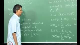
Let A be a positive-definite matrix. We can define an inner product in Rn by:
⟨u,v⟩ =uTAv.
This is called a weighted inner product and often appears in structural analysis:
• A: stiffness matrix
• u,v: displacement vectors.
Such inner products reflect physical energy-like quantities, for instance:
Strain Energy = uTKu / 2,
Where K is the stiffness matrix of the structure.
Detailed Explanation
The matrix representation of inner products allows us to generalize the concept, making it applicable in various real-world scenarios such as structural analysis. By using a positive-definite matrix A (often representing stiffness in engineering), the inner product can be computed as a quadratic form, providing insights into the physical behavior of structures. Calculating strain energy can be linked back to these inner products, demonstrating how mathematical concepts are deeply intertwined with physical interpretations.
Examples & Analogies
Imagine weighing items in a balance. Each object (displacement vector) contributes differently based on its material and shape (weighting matrix). The matrix representation helps engineers assess the structural integrity of materials under stress, just as balance scales determine whether items are well supported. This highlights the critical balance engineers must manage when designing robust structures.
Bessel’s Inequality and Parseval’s Identity
Chapter 16 of 18
🔒 Unlock Audio Chapter
Sign up and enroll to access the full audio experience
Chapter Content
Let {e1,e2,...,en} be an orthonormal set in V, and let v ∈V.
Bessel’s Inequality:
Σ |⟨v,ei⟩|² ≤ ∥v∥²
for i from 1 to n.
Parseval’s Identity (when set is complete):
Σ |⟨v,ei⟩|² = ∥v∥²
for i from 1 to ∞.
These identities are fundamental in analyzing signals, waveforms, and deflections using series expansions in Civil Engineering.
Detailed Explanation
Bessel's Inequality provides an upper bound on the sum of the squared inner products of a vector with an orthonormal set, indicating that the contributions of all basis vectors cannot exceed the square of the vector's norm. On the other hand, Parseval's Identity establishes equality when the orthonormal set is complete, revealing that the vector can be completely reconstructed from its projections in a perfect system. These identities are vital in signal processing and analytical modeling, helping to understand behaviors in systems across engineering disciplines.
Examples & Analogies
Imagine a musician's full performance is captured in separate audio tracks (orthonormal sets). Bessel's Inequality shows that the total 'volume' of the sound (energy of performances) does not exceed the original recording's potential. In a complete set of tracks (Parseval’s Identity), all melodies harmonize together perfectly without confusion. This reflects how engineers must ensure their designs maintain stability and functionality, just as musicians ensure their pieces are cohesive.
Hilbert Spaces (Advanced)
Chapter 17 of 18
🔒 Unlock Audio Chapter
Sign up and enroll to access the full audio experience
Chapter Content
A Hilbert space is a complete inner product space. That is, every Cauchy sequence in the space converges to a point within the space.
• ℓ²: space of square-summable sequences.
• L²[a,b]: space of square-integrable functions.
Hilbert spaces form the theoretical backbone of elasticity theory, fluid dynamics, and variational methods in Civil Engineering.
Detailed Explanation
Hilbert spaces extend the notion of inner product spaces into realms where completeness is a defining characteristic. Completeness refers to the property that any Cauchy sequence (a sequence whose elements become arbitrarily close) converges within the space itself. Examples include spaces of sequences and functions that satisfy certain integrability conditions. Hilbert spaces are foundational in theoretical frameworks across various disciplines in engineering, particularly in understanding complex systems like elasticity and fluid dynamics.
Examples & Analogies
Picture a network of roads leading to a town where all highways converge (completeness). Just like all paths lead to the town, every Cauchy sequence in a Hilbert space leads to a specific point (convergence). In civil engineering, understanding fluid dynamics is akin to studying the flow of water through these roads—each flow must find its way naturally and efficiently through the network, ensuring systems behave predictably.
Computational Perspective
Chapter 18 of 18
🔒 Unlock Audio Chapter
Sign up and enroll to access the full audio experience
Chapter Content
In real-world engineering software like ANSYS, ABAQUS, or STAAD.Pro:
• Inner products are used in assembling matrices (mass, stiffness).
• Orthogonalization methods (Gram-Schmidt, QR) are used for solving large systems.
• Norms are used for convergence criteria in simulations.
• Projections help with error minimization in numerical modeling.
Understanding the mathematical foundation of these methods enhances the engineer’s ability to interpret, verify, and improve simulation results.
Detailed Explanation
In practical engineering applications, sophisticated software utilizes inner product concepts to optimize structural analyses. Inner products facilitate matrix assembly by encoding relationships between components, while orthogonalization methods streamline computations needed for solving large systems efficiently. Norms contribute significantly to determining stability and convergence in simulations, while projections minimize errors by ensuring approximations are as close to actual values as possible. A thorough understanding of these foundations is crucial for engineers to enhance their designs and validate results effectively.
Examples & Analogies
Imagine a chef preparing a complex dish, with each ingredient requiring precise measurements and methods to achieve the best flavor. The software acts like a master chef in analyzing engineering designs, combining inner products (ingredients) to produce optimal structures. Just as chefs must know how to adjust flavors based on testing (norms and projections), engineers use these tools to fine-tune their models, ensuring they stand the test of real-world challenges.
Key Concepts
-
Vector Spaces: Fundamental constructs where vectors exist and operations can be performed.
-
Inner Product: A crucial operation that allows for the measurement of angles and lengths in vector spaces.
-
Orthogonality: The condition of two vectors being perpendicular in terms of their inner product being zero.
-
Norm: A representation of vector length derived from the inner product.
-
Projection: The method of expressing one vector in terms of another, essential in least squares.
-
Cauchy-Schwars Inequality: A fundamental inequality crucial for understanding vector relationships.
Examples & Applications
In Euclidean space R², the inner product is defined as ⟨u,v⟩ = u1v1 + u2v2. This allows us to compute angles and distances easily.
In the space of continuous functions C[a,b], the inner product is given by ⟨f,g⟩ = ∫(f(x)g(x)) dx from a to b, applicable in various engineering fields.
Memory Aids
Interactive tools to help you remember key concepts
Rhymes
To know your space, define it well, an inner product ring a bell. Angle and length it will bring, vectors dance with angles sing.
Stories
Once in a vector land, two friends met at a right angle, their bond was strong as they never tangled, together they formed a powerful space.
Memory Tools
Remember LCP: Linearity, Conjugate, Positive to define inner space correctly.
Acronyms
Use 'IPA' to recall Inner Product Algebra
Inner product
Projections
and Application.
Flash Cards
Glossary
- Inner Product
A function that associates a pair of vectors in a vector space with a scalar, satisfying specific properties.
- Orthogonal
Two vectors are orthogonal if their inner product is zero.
- Orthonormal
A set of vectors that are orthogonal and of unit length.
- Projection
The representation of a vector in the direction of another vector.
- Norm
A function that assigns a positive length or size to a vector.
- Cauchy–Schwarz Inequality
An inequality that states |⟨u, v⟩| ≤ ||u||·||v|| for any vectors u and v.
- Triangle Inequality
For any vectors u and v, ||u + v|| ≤ ||u|| + ||v||.
Reference links
Supplementary resources to enhance your learning experience.