
Density Variation and Mass Flux
Enroll to start learning
You’ve not yet enrolled in this course. Please enroll for free to listen to audio lessons, classroom podcasts and take practice test.
Interactive Audio Lesson
Listen to a student-teacher conversation explaining the topic in a relatable way.
Incompressible Flow Basics
🔒 Unlock Audio Lesson
Sign up and enroll to listen to this audio lesson

Today, we will discuss incompressible flow. Does anyone know what it means when we say a flow is incompressible?

Does it mean that the density of the fluid doesn't change?
Exactly! In incompressible flow, especially when the Mach number is below 0.3, we treat the density as constant. This simplifies a lot of our calculations.

Why is Mach number important?
Good question! The Mach number indicates whether the speeds are close to the speed of sound, which helps in deciding whether density changes are significant. Can anyone define it?

It's the ratio of the speed of the flow to the speed of sound in that medium.
Exactly! Now, can anyone recall what happens under incompressible flow conditions?

I think we can use mass flow equations without worrying about density changes.
That's right! Let's summarize: When the Mach number is less than 0.3, we simplify the density to a constant, which helps us apply mass conservation principles more easily.
Mass Flux vs. Volumetric Flux
🔒 Unlock Audio Lesson
Sign up and enroll to listen to this audio lesson

Now that we understand incompressible flow, let’s talk about mass flux versus volumetric flux. Who can explain the difference?
Isn't mass flux related to mass flow rate, while volumetric flux is just the volume flowing per unit time?
Yes! Mass flux is generally expressed as density times velocity and gives us mass flow rate, while volumetric flux is simply the product of area and velocity. So, if we consider **Q = A * V**, we represent volumetric flow.
What if density actually changed?
Great point! If density changes are significant, we need to treat both density and velocity separately in our equations. Can you give an example where that might be necessary?
In high-speed flows, like in nozzles or diffusers!
Exactly! We'll keep that in mind as we continue. Always remember, under incompressible flow, we assume density is constant which simplifies our calculations with mass conservation equations.
Importance of Velocity Profiles
🔒 Unlock Audio Lesson
Sign up and enroll to listen to this audio lesson
Next, let's discuss how velocity profiles impact our computations in fluid dynamics. Why do you think understanding velocity distribution is crucial?
I think it helps us determine how much fluid is actually flowing through a cross-section.
Exactly! For pipe flows, velocity is zero at the wall and peaks at the center. What happens if we assume uniform velocity?
We might underestimate or overestimate the actual flow rate!
Right! We often deal with average velocities, which can be derived through integrals of the velocity profile over the cross-section. Anyone familiar with how we can calculate average velocity from a varying profile?
We can use surface integrals and apply the average formula?
Correct! Understanding velocity distribution not only allows us to compute mass flux accurately but is essential in practical applications, such as designing pipe systems.
Applying Conservation of Mass
🔒 Unlock Audio Lesson
Sign up and enroll to listen to this audio lesson
Now let’s look at how to apply mass conservation equations practically. Can anyone summarize the steps we should take?
First, classify the flow type—like one-dimensional or steady, right?
Exactly! Then we identify the control volume and analyze the inflow and outflow. What happens next?
We should write out the mass balance equation and solve it according to the known variables!
Perfect! Let’s consider an example: A tank with inflows only. If we know the velocities and cross-sectional areas, can we calculate the change in water height over time?
We can substitute the values into the mass balance equation and solve for the height change!
Correct! Remember, mass conservation is fundamental in fluid dynamics, and being able to apply these principles in various scenarios is key. Practice is essential!
Introduction & Overview
Read summaries of the section's main ideas at different levels of detail.
Quick Overview
Standard
The section introduces the concept of incompressible flow, stating that when the Mach number is below 0.3, the density variation is negligible. This allows for the simplification of mass conservation equations into volumetric flow equations, emphasizing the importance of understanding velocity profiles in control volumes and various flow scenarios.
Detailed
Detailed Summary
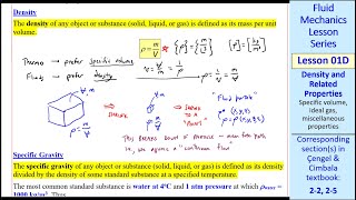
In fluid mechanics, the density variation and mass flux are critical concepts, especially when considering incompressible flow. When the Mach number (Ma) is less than 0.3 — which applies to both gases and liquids — the variation in density is minimal enough to be considered negligible. This allows us to assume that density remains constant within the flow, thus simplifying calculations considerably.
The primary relationship highlighted in this section is between mass flux and volumetric flux, formulated through mass conservation equations. Here,
- The volumetric flux (Q) can be equated to the product of area (A) and velocity (V) under the assumption of constant density. This results in the relationship Q = A * V, where the inflow and outflow are analyzed within a control volume, typically leading to unsteady flow calculations.
Significantly, understanding how velocity varies within a control volume is vital for solving real-world fluid dynamics problems, specifically when the flow is not uniform. The section emphasizes that accurately classifying flow conditions (one-dimensional, laminar, fixed control volume, etc.) is crucial to applying the Reynolds transport theorem correctly.
Various examples illustrate the application of these concepts, such as calculating changes in water height in tanks and analyzing flow characteristics in rivers, showcasing how theoretical concepts translate into practical assessments.
Youtube Videos


Audio Book
Dive deep into the subject with an immersive audiobook experience.
Incompressible Flow Assumption
Chapter 1 of 4
🔒 Unlock Audio Chapter
Sign up and enroll to access the full audio experience
Chapter Content
When the flow systems have a Mach number less than 0.3, we can assume the flow is incompressible. This means that even though density varies, the variation is negligible compared to other components, allowing us to treat density as constant.
Detailed Explanation
In fluid dynamics, the Mach number (Ma) gives us an idea of the speed of the flow compared to the speed of sound in that medium. When Ma is less than 0.3, the flow is typically treated as incompressible. Since the changes in density are very small, we can simplify our calculations by assuming that density remains constant throughout the fluid. This simplification helps in solving fluid problems more easily, as we no longer need to account for density fluctuations.
Examples & Analogies
Think of a river with a mild current—here, the water density remains mostly constant as it flows, allowing engineers to use simpler calculations to analyze its flow. However, if the river flows over a waterfall or has a strong rapids, the density might vary due to bubbles and changes in pressure, making it more complex to analyze.
Mass and Volumetric Flux
Chapter 2 of 4
🔒 Unlock Audio Chapter
Sign up and enroll to access the full audio experience
Chapter Content
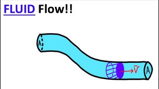
In cases of incompressible flow with constant density, mass flux can be expressed as volumetric flux. When we multiply the velocity of the flow by the cross-sectional area (A), we get the volumetric flow rate (Q): Q = A * V.
Detailed Explanation
Mass flux is the rate of mass flow per unit area, while volumetric flux is concerned with the volume of fluid passing through a section per unit time. For incompressible flows, when density is constant, we can simplify mass calculations by expressing them in terms of volumetric flow. Thus, Q = A * V, where A is the cross-section of the fluid and V is the average velocity. This equation allows engineers to predict how much fluid will flow through a section of a pipe in a given time.
Examples & Analogies
Imagine a garden hose: the amount of water flowing out depends on how wide the nozzle is (area) and how hard you squeeze the trigger (velocity). If you know the width of the nozzle and how fast the water is flowing, you can easily calculate how much water will exit over time, similar to calculating volumetric flux.
Velocity Field and Control Volume
Chapter 3 of 4
🔒 Unlock Audio Chapter
Sign up and enroll to access the full audio experience
Chapter Content
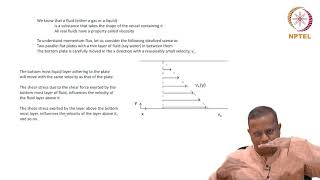
To apply the mass conservation equation effectively, one must understand the velocity field and how velocity varies across the control surface. Knowing whether the flow is one-dimensional or requires a more complex model based on varying velocity fields is crucial for accurate calculations.
Detailed Explanation
In fluid dynamics, the velocity field describes how the velocity of fluid particles varies in space. When analyzing fluid flow, especially in complex systems like pipes or channels, it is important to determine if the flow can be approximated as one-dimensional or if it varies significantly across the cross-section. The mass conservation equation depends heavily on this understanding, as it ensures continuity of mass as fluid flows into and out of a control volume (a designated area to analyze flow).
Examples & Analogies
When you're paddling a kayak down a river, the speed of the water varies depending on where you are—near the edges, the water is slower due to friction with the bank; in the middle, it's faster. By mapping out this velocity distribution, you can adjust your paddling to navigate effectively, just as engineers must model velocity fields to understand flow dynamics accurately.
Average Velocity and Discharge Calculation
Chapter 4 of 4
🔒 Unlock Audio Chapter
Sign up and enroll to access the full audio experience
Chapter Content
When dealing with flows that don't have a uniform velocity distribution, engineers often calculate average velocity by integrating over the area. The average velocity then allows for accurate discharge calculations, which represent the total flow out of a system.
Detailed Explanation
In practical applications, the velocity of fluid does not always remain constant across a cross-sectional area; it can vary due to several factors like friction. To find the average velocity, engineers use calculus to integrate the velocity profile over the area, which gives a representative value for calculating discharge. Discharge measures how much fluid is flowing through a specific area of the system per unit time.
Examples & Analogies
Consider drinking through a straw. If the bottom of the straw is uneven or bent, the speed of the liquid flowing through different parts of the straw changes. If you want to know the average amount of soda you're sipping, you would consider the entire straw's cross-section and how much fluid flows through it, much like calculating average velocity in a fluid system.
Key Concepts
-
Incompressible Flow: Fluid density remains constant for flow situations where Mach number is less than 0.3.
-
Mass Flux: Defined as the mass flow rate per unit area, critical for analyzing inflows and outflows.
-
Volumetric Flux: The volume flow rate of a fluid, calculated using area and velocity under certain assumptions.
-
Reynolds Transport Theorem: A principle to relate mass transfer within a control volume to its boundaries.
Examples & Applications
Example 1: Calculating the discharge from a tank with multiple inflows.
Example 2: Analyzing flow velocity distribution in a pipe.
Memory Aids
Interactive tools to help you remember key concepts
Rhymes
Incompressible flow, density's the same, keep it quite simple, that's the game.
Stories
Imagine a river flowing steadily, where every drop of water is in sync, as if choreographed, showing us that under low speeds, density doesn’t change, making calculations a breeze!
Memory Tools
Remember the acronym MIST: M for Mass flux, I for Incompressible flow, S for Speed (Mach number), T for Transport Theorem.
Acronyms
Use **D-V**
for Density
for Volumetric flow
to remember their role in fluid equations.
Flash Cards
Glossary
- Incompressible Flow
A flow condition where the fluid density is assumed constant despite changes in pressure or temperature.
- Mach Number
The ratio of the speed of a fluid to the speed of sound in that fluid.
- Mass Flux
The mass flow rate of a substance per unit area.
- Volumetric Flux
The volume flow rate of a fluid per unit area.
- Reynolds Transport Theorem
A fundamental theorem in fluid dynamics that relates the change of mass within a control volume to the flow of mass across its boundaries.
- Velocity Profile
The distribution of velocity across a flow section, usually varies from zero at the boundary to a maximum value at the center.
Reference links
Supplementary resources to enhance your learning experience.