
Velocity Distribution in Pipe Flow
Enroll to start learning
You’ve not yet enrolled in this course. Please enroll for free to listen to audio lessons, classroom podcasts and take practice test.
Interactive Audio Lesson
Listen to a student-teacher conversation explaining the topic in a relatable way.
Incompressible Flow and Mach Number
🔒 Unlock Audio Lesson
Sign up and enroll to listen to this audio lesson

Today, we’re exploring velocity distribution in pipe flow. Can anyone tell me when we can treat fluid flow as incompressible?

Isn't it when the Mach number is less than 0.3?
Exactly! When the Mach number is below 0.3, we can ignore density changes. Can anyone explain why that’s significant?

Because it simplifies the equations we use, right? We can treat the density as constant.
Absolutely! This simplification is crucial for deriving mass conservation equations. Remember, 'Low Ma Equals Simple Flows, or LMa=SF' could be a useful mnemonic!
Volumetric Flux and Mass Conservation
🔒 Unlock Audio Lesson
Sign up and enroll to listen to this audio lesson

Now let's discuss volumetric flux. Who remembers the formula that relates area, velocity, and discharge?

I think it's Q = A * V, where Q is the discharge.
Correct! And how does this play into mass conservation?

By assuming density is constant, we can simplify mass conservation into volumetric terms?
Spot on! This transition from mass to volumetric flux is vital for practical calculations in fluid mechanics. Let’s not forget our mnemonic 'VAD – Volumetric Assumption for Density!'
Velocity Distribution Across Pipe Sections
🔒 Unlock Audio Lesson
Sign up and enroll to listen to this audio lesson
How does velocity distribution typically vary in a pipe?
I believe it’s zero at the walls and maximum at the center?
Precisely! This concept is crucial for determining flow behavior. Can anyone explain how we can calculate average velocity from this distribution?
By integrating the velocity over the cross section?
Exactly! This integration provides a holistic view of how the flow behaves through the entire pipe. Remember, 'Pipe Flow = Max V at Center, or PF=MV@C' can help with this concept!
Introduction & Overview
Read summaries of the section's main ideas at different levels of detail.
Quick Overview
Standard
In this section, the concept of velocity distribution in pipe flow is explored, particularly under conditions of incompressible flow where density is assumed constant. It details the relationship between velocity and cross-sectional area, introducing key equations related to mass and volumetric flux while addressing the significance of velocity variation in analyzing flow systems.
Detailed
Velocity Distribution in Pipe Flow
This section delves into the characteristics of velocity distribution in fluid flows, particularly in incompressible scenarios where the Mach number (Ma) is less than 0.3. Under these conditions, density variations within the fluid are negligible, allowing us to treat fluid behavior as incompressible. Given this assumption, key concepts such as volumetric flux and mass conservation equations are simplified, where the density becomes a constant factor.
The fundamental equations presented include the relationship between volumetric flux
\[ Q = A imes V \]
where Q represents discharge, A is the cross-sectional area, and V is velocity. This approach permits the analysis of real-world pipe flow problems by establishing relationships between velocity distributions, particularly illustrating the variation of velocity from zero at the pipe walls to maximum at the center.
The importance of understanding velocity distributions is emphasized, as it directly impacts calculations involving mass conservation in fluid mechanics. Simplified assumptions regarding velocity fields facilitate the resolution of complex flow problems, guiding the application of mass conservation principles through Reynolds transport theorem and aiding in the integration of surface and volumetric elements in analysis.
Youtube Videos


Audio Book
Dive deep into the subject with an immersive audiobook experience.
Incompressible Flow Assumption
Chapter 1 of 5
🔒 Unlock Audio Chapter
Sign up and enroll to access the full audio experience
Chapter Content
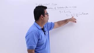
When you have any flow systems, mach number less than 0.3, so we can use flow as incompressible flow, density does not vary significantly. So, density becomes constant, as density becomes constant, as you know it, it is very simplified problem what we are going to solve.
Detailed Explanation
In fluid dynamics, we often come across situations where we can simplify the behavior of fluids. One such simplification arises when the flow of a fluid is deemed incompressible. This occurs when the mach number (a measure of flow speed relative to the speed of sound in the fluid) is less than 0.3. Under these conditions, changes in density are minimal enough that we can assume it to be constant. This assumption makes mathematical equations and problem-solving much easier since we can treat the properties of the fluid as unchanging and apply simplified models.
Examples & Analogies
Consider a water hose connected to a faucet. When you turn on the faucet, the water flows quickly through the hose, but the speed is low enough that we can consider the water's density unchanged (incompressible). As a result, we can apply simpler equations to analyze how the water moves from the faucet through the hose.
Volumetric Flux vs. Mass Flux
Chapter 2 of 5
🔒 Unlock Audio Chapter
Sign up and enroll to access the full audio experience
Chapter Content
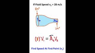
So, instead of the mass flux we are now talking about volumetric flux. That means, if you multiply the velocity into area, then what you get is unit volume per unit height, volumetric flux.
Detailed Explanation
In fluid flow analysis, we often differentiate between two types of flow measurements: mass flux and volumetric flux. Mass flux is the mass of fluid passing through a given area per unit time, while volumetric flux measures the volume of fluid passing through a given area per unit time. When density is taken to be constant (as in the case of incompressible flow), we can express mass flux in terms of volumetric flux, leading us to the relationship Q = AV, where Q is discharge (volumetric flow rate), A is cross-sectional area, and V is flow velocity.
Examples & Analogies
Think about filling a large tub with water. The volumetric flux can be thought of as how much water is entering the tub every minute (like a bucket's worth of water). If you know the area of the tub opening and the speed of the water flowing in, you can easily calculate how fast the tub is filling up without worrying about the weight of the water.
Velocity Distribution in Pipe Flow
Chapter 3 of 5
🔒 Unlock Audio Chapter
Sign up and enroll to access the full audio experience
Chapter Content
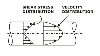
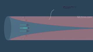
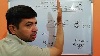
As we discussed earlier, the velocity will be 0 near the wall, velocity will be maximum at the center and so there will be velocity distribution, there will be velocity distribution from this side.
Detailed Explanation
In a pipe flow situation, the velocity of the fluid does not remain constant across the entire cross-section of the pipe. The fluid moves more slowly near the walls of the pipe due to friction. In contrast, the fluid in the center of the pipe experiences less friction and flows faster. This creates a velocity profile where the velocity is highest in the center and decreases to zero at the pipe walls (the 'no-slip condition'). Understanding this velocity distribution is crucial for predicting how the fluid behaves and how to design systems involving fluid flow efficiently.
Examples & Analogies
Imagine a crowded hallway. When people are walking, those in the center of the hallway move quickly, while those near the walls might slow down or stop to avoid bumping into others. Similarly, in a pipe, fluid particles in the center can move freely, while those near the edges are impeded by friction against the pipe walls.
Importance of Velocity Field Knowledge
Chapter 4 of 5
🔒 Unlock Audio Chapter
Sign up and enroll to access the full audio experience
Chapter Content
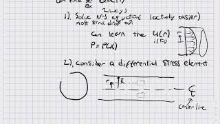
To solve this mass conservation equation I should have knowledge on velocity field.
Detailed Explanation
In fluid mechanics, to apply the mass conservation equation effectively, it is vital to understand how the velocity field behaves. This involves knowing whether the velocity is uniform or varies with position in the given system. If the velocity distribution is uniform, calculations are more straightforward, but real-world situations usually involve varying velocities based on flow conditions and fluid properties. Determining the velocity field allows for accurate predictions about mass flow rates and the behavior of fluids under various conditions.
Examples & Analogies
When planning a road trip, knowing the speed limits and traffic patterns on different sections of your route can help you estimate your travel time. Similarly, understanding the velocity field in fluid mechanics enables engineers to predict how quickly fluids will move in pipes or ducts, which is essential for efficient system design.
Average Velocity Calculation
Chapter 5 of 5
🔒 Unlock Audio Chapter
Sign up and enroll to access the full audio experience
Chapter Content
Once you know the average velocity you multiply with the area you will get the volumetric flux or the discharge.
Detailed Explanation
When dealing with fluid flow, calculating the average velocity is important, especially when the velocity distribution is not uniform. By integrating the velocity across the flow area or using values provided in a problem, we can determine the average velocity. When this average is multiplied by the cross-sectional area of the flow, we can find the discharge (volumetric flow rate), indicating how much fluid passes through a given point per unit time.
Examples & Analogies
Consider a garden sprinkler with multiple small holes, each watering a different area of the lawn. If you want to determine how much water is used overall, you would measure the rate of water coming out of each hole and calculate the average rate of flow across all holes, combined with the total area they cover.
Key Concepts
-
Incompressible Flow: Assumed where density changes are negligible; simplifies calculations.
-
Volumetric Flux: Direct relationship between area, velocity, and flow rate.
-
Velocity Distribution: Varies from zero at walls to maximum at the center; critical in flow analysis.
-
Mass Conservation: Fundamental principle affecting flow dynamics; connects inflow and outflow.
-
Reynolds Transport Theorem: A tool for analyzing changes in mass within control volumes.
Examples & Applications
In a pipe with a diameter of 0.5m operating at a velocity of 3 m/s, the volumetric flow rate can be calculated as Q = A * V = π(0.5/2)^2 * 3.
Using average velocity from integration, if the velocity across the cross-section varies, compute using ∫V dA/A to find effective velocity.
Memory Aids
Interactive tools to help you remember key concepts
Rhymes
Incompressible flow, simple as can be, Mach less than point three equals less density.
Stories
Imagine a pipe where water flows fast, at the center it's quick, at the walls, it won't last. In and out we measure, keeping track is the key, for flow rate and mass, as easy as A-B-C!
Memory Tools
Think 'VAQ': Velocity, Area equals Quantity (flow rate).
Acronyms
RTP
Remember The Pipe - Velocity is highest in the center
zero at the walls.
Flash Cards
Glossary
- Incompressible Flow
A flow regime where density variations within the fluid are negligible, often treated as constant.
- Mach Number
A dimensionless number representing the ratio of the speed of a fluid to the speed of sound in that fluid.
- Volumetric Flux
The volume of fluid that flows through a given cross-sectional area per unit time, typically expressed as Q = A * V.
- Mass Conservation Equation
An equation that states mass cannot be created or destroyed in an isolated system, leading to the relationship between inflow and outflow.
- Reynolds Transport Theorem
A principle that relates the change in a quantity transported by a flow to its inflow and outflow across control volumes.
Reference links
Supplementary resources to enhance your learning experience.