
Boundary Conditions and Solutions
Enroll to start learning
You’ve not yet enrolled in this course. Please enroll for free to listen to audio lessons, classroom podcasts and take practice test.
Interactive Audio Lesson
Listen to a student-teacher conversation explaining the topic in a relatable way.
Introduction to Boundary Layer Approximations
🔒 Unlock Audio Lesson
Sign up and enroll to listen to this audio lesson

Good morning, class! Today, we’re diving into boundary layer approximations. Can anyone explain what a boundary layer is?

Isn't it the thin layer of fluid at a solid surface where the velocity changes relatively rapidly?
Exactly! It’s the region where the effects of viscosity are significant. We typically focus on how to approximate fluid behavior in this layer, especially using the Navier-Stokes equations.

What about the equations? How do we derive them?
Great question! We derive the boundary layer equations by simplifying the Navier-Stokes equations under specific assumptions. Can anyone recall these assumptions?

Assuming two-dimensional and incompressible flow!
Correct! We'll use these conditions to derive key equations. Let’s summarize the mass conservation equation: it states that the divergence of velocity must equal zero in steady-state flow.
Boundary Layer Equations
🔒 Unlock Audio Lesson
Sign up and enroll to listen to this audio lesson

Now, moving on to the boundary layer equations, we can express them in parabolic form. Can anyone tell me why parabolic form is helpful?

They simplify our calculations compared to the full Navier-Stokes equations.
Exactly! They allow us to find solutions more efficiently. The parabolic equations provide us with velocity profiles within the boundary layer. Let’s also discuss the non-slip conditions at the wall.
So at the wall, the velocities should be zero?
Right! That’s the essence of the no-slip condition. It dictates how the fluid interacts with the surface. Now, what do you think happens at the free stream boundary?
That’s where the flow velocity equals the free stream velocity.
Correct. We’ll leverage these conditions for our later calculations.
Displacement and Momentum Thickness
🔒 Unlock Audio Lesson
Sign up and enroll to listen to this audio lesson
Next, let's cover displacement thickness and momentum thickness. Why do we need to define these concepts?
To understand the mass and momentum deficit caused by wall effects?
Indeed! Displacement thickness quantifies the shift of the streamline outward due to the boundary layer. Can someone summarize how we mathematically derive this thickness?
We integrate the velocity profile to find how much slower the flow is within the boundary layer compared to the free stream.
Exactly! Do you all remember the formula to calculate it?
Yes, it’s integrating 1 minus the ratio of velocity to free stream over the y direction!
Good job! And momentum thickness is another important measure linked to drag forces. Let's elaborate on how it impacts friction on surfaces.
Understanding Turbulent Flow
🔒 Unlock Audio Lesson
Sign up and enroll to listen to this audio lesson
Now, let’s shift towards turbulent flows, which are much more complicated than laminar flows. What main differences can you identify?
Turbulent flows are chaotic and have higher shear stress at the surface?
Spot on! They are not dictated solely by viscosity but rather by a complex interplay of multiple factors. Can anyone relate why empirical equations are used in predicting turbulent flows?
Since turbulent flows are too complex for exact equations, we rely on experimental data to fit empirical models?
Exactly! We use simplified relationships like the one-seventh power law to describe velocity profiles. Understanding these concepts helps in designing engineering solutions. Can anyone provide a context where this might apply?
In designing aircraft wings to reduce drag, for instance!
Great example! Let's summarize the key takeaways from today’s class.
Introduction & Overview
Read summaries of the section's main ideas at different levels of detail.
Quick Overview
Standard
In this section, we delve into the fundamentals of boundary layer approximations, particularly for laminar flows. It addresses boundary layer equations derived from Navier-Stokes principles, the significance of the displacement thickness, and momentum thickness, while also discussing how numerical methods play a role in finding solutions to these equations.
Detailed
Detailed Summary
In this chapter on Fluid Mechanics, the discussion centers around boundary layer approximations, vital for understanding fluid flow characteristics near solid surfaces. It begins with the derivation of boundary layer equations from the Navier-Stokes equations, particularly the mass conservation and momentum equations for laminar flows.
Key topics include:
- Boundary Layer Equations: Simplifications lead to parabolic equations which facilitate the calculation of layer thickness, wall shear stress, and friction coefficients. The non-slip boundary conditions at the wall and free stream conditions are critical in these calculations.
- Displacement Thickness: This concept captures the effect of boundary layers on the flow, quantitatively representing how much the streamline is deflected due to the velocity differential within the boundary layer. Mathematical formulations are provided to compute displacement thickness.
- Momentum Thickness: Closely related to shear stress on the plate, this thickness quantifies the loss of momentum within the flow due to boundary layer effects.
- Laminar vs. Turbulent Flows: The section differentiates between laminar and turbulent boundary layers, with an emphasis on empirical equations and approximations used in turbulence studies.
The importance of computational techniques, historical background regarding significant contributors like Prandtl, and the methodologies used illustrate the development of fluid dynamics concepts over time.
Youtube Videos


![[CFD] Convection (Heat Transfer Coefficient) Boundary Conditions](https://img.youtube.com/vi/ygR31_vhvJI/mqdefault.jpg)

![[CFD] Pressure-Inlet Boundary Conditions](https://img.youtube.com/vi/Er2j5Kq17as/mqdefault.jpg)
Audio Book
Dive deep into the subject with an immersive audiobook experience.
Introduction to Boundary Layer Approximations
Chapter 1 of 7
🔒 Unlock Audio Chapter
Sign up and enroll to access the full audio experience
Chapter Content
Let us discuss boundary layer approximations based on the previous classes. We derived boundary layer equations as approximations of Navier-Stokes equations near boundary layer formations for flow past a flat plate. Today, we will explore numerical solutions of these boundary layer equations.
Detailed Explanation
In this section, the professor introduces the concept of boundary layer approximations, emphasizing their relevance for fluid flow over surfaces like flat plates. Boundary layers occur due to the effects of viscosity, causing a variation of velocity from the boundary (the surface of the plate) into the fluid away from the surface. The primary focus will be how to numerically solve these equations, which is an essential skill in fluid mechanics.
Examples & Analogies
Imagine driving a car on a smooth highway. As you speed up, air pushes against the hood but barely touches the sides. The air closest to the car moves slower due to friction, while the air further away moves faster. This is analogous to how boundary layers form along the surface of a flat plate, where the fluid experiences different velocities based on its proximity to the plate.
Mass and Momentum Conservation in Boundary Layers
Chapter 2 of 7
🔒 Unlock Audio Chapter
Sign up and enroll to access the full audio experience
Chapter Content
Boundary layer equations are derived from mass conservation and linear momentum equations. For two-dimensional incompressible flow, the continuity equation states that the rate of change of mass must equal zero, leading to specific forms of equations for boundary layers.
Detailed Explanation
Here, the professor discusses how to derive the boundary layer equations using the principles of mass and momentum conservation. The continuity equation implies that if there is no mass entering or exiting a specific volume of fluid, the amount of fluid must remain constant. In boundary layers, this means we define equations that help calculate how fluid velocities change from the wall into the main flow, leading us to calculate key parameters like velocity distributions and boundary layer thickness.
Examples & Analogies
Think of a crowd of people (the fluid) moving through a narrow entrance (the boundary). As people approach the entrance, they slow down (boundary condition) while others who are further away from the entrance continue moving at normal speed. The convergence and divergence of this crowd mimic how fluid behaves in a boundary layer.
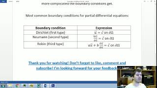
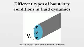
Defining Boundary Conditions
Chapter 3 of 7
🔒 Unlock Audio Chapter
Sign up and enroll to access the full audio experience
Chapter Content
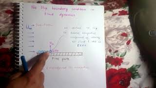
Specific boundary conditions are set, such as the velocity of fluid being zero at the wall (non-slip condition) and the known velocity at the free stream. These conditions help in solving boundary layer equations numerically.
Detailed Explanation
Boundary conditions are crucial in solving differential equations like those governing fluid flow. The no-slip condition at a wall means that the fluid velocity exactly at the surface of the wall is zero, indicating that there is no movement of fluid relative to the surface. At the same time, we know the speed of the fluid as it moves further away from the surface in the free stream. This combination of conditions allows for the correct computations of how fluid moves towards and away from the surface.
Examples & Analogies
Picture yourself sliding down a slide at a park. When you touch the slide, you come to a complete stop because there's no movement at the point of contact; this is like the non-slip condition. However, as you move further away from the slide (into the air), you feel the wind pushing against you, similar to how fluid velocities are established in the free stream.
Computational Techniques in Fluid Dynamics
Chapter 4 of 7
🔒 Unlock Audio Chapter
Sign up and enroll to access the full audio experience
Chapter Content
Modern computational techniques allow us to solve boundary layer equations rapidly compared to historical methods. Numerical solutions can be derived using advanced computing resources, facilitating analysis of complex fluid flows.
Detailed Explanation
Today's computational fluid dynamics (CFD) techniques enable us to tackle complex fluid behavior that would have been exceedingly difficult to analyze manually. By implementing numerical methods, we can simulate and calculate how fluids behave under various conditions and geometries. This capability is a huge advancement compared to manual methods developed over a century ago.
Examples & Analogies
Think about how navigation has evolved. Initially, sailors relied on maps and stars (manual calculations) to navigate the seas, which was tedious and error-prone. Today, GPS systems use satellites and complex algorithms (computational techniques) to provide accurate positioning and routing in real-time, reflecting how boundary layer equations can now be solved much more efficiently.
Understanding Displacement Thickness
Chapter 5 of 7
🔒 Unlock Audio Chapter
Sign up and enroll to access the full audio experience
Chapter Content
Displacement thickness arises due to the effect of boundary layer formations, where streamlines are deflected in the presence of a flat plate. It quantifies how much the actual streamline deviates from a no-boundary-layer condition.
Detailed Explanation
Displacement thickness provides insight into the 'thickness' of the boundary layer by measuring how much the effective flow profile is shifted due to the presence of the boundary layer. As fluid moves over a boundary, the proximity to the wall alters velocity, displacing the flowing fluid away from the wall. Displacement thickness is significant in understanding the flow's behavior and calculating forces acting on surfaces.
Examples & Analogies
Imagine a river flowing over a rock. The water flowing closest to the rock moves slowly due to friction, while water further out flows more freely. This results in a 'displacement' of the water surface, similar to how displacement thickness shifts the effective flow profile due to boundary layers.
Momentum Thickness and Its Implications
Chapter 6 of 7
🔒 Unlock Audio Chapter
Sign up and enroll to access the full audio experience
Chapter Content
Momentum thickness is related to the shear stresses acting on the surface of the plate resulting from the boundary layers. It is defined as the reduction in momentum at the boundary layer due to the velocity difference across the layer.
Detailed Explanation
Momentum thickness helps quantify how the velocity profile inside the boundary layer differs from that outside. It reflects the impact of the boundary layer on drag forces acting on a surface. Like displacement thickness, it reveals how much effective flow is altered because of viscosity and friction.
Examples & Analogies
Think of a heavy blanket lying on top of a bed. While the blanket (representing the boundary layer) may seem insignificant at a glance, it actually alters how easily you can fold the blanket back (analogous to how momentum thickness alters movement of fluid), showing that even small factors can have a substantial impact on a larger system.
Analyzing Turbulent Boundary Layers
Chapter 7 of 7
🔒 Unlock Audio Chapter
Sign up and enroll to access the full audio experience
Chapter Content
Turbulent boundary layers involve chaotic and fluctuating flow patterns, requiring empirical approximations for their analysis. Unlike laminar flows, turbulent flows can be represented by average characteristics derived from experimental data.
Detailed Explanation
Turbulent boundary layers are much more complex due to the irregular and chaotic nature of the flow within these layers. Instead of straightforward equations, empirical relationships based on experiments give approximations of how these turbulent layers behave. Understanding these flows is crucial, especially in engineering applications where they influence drag and lift.
Examples & Analogies
Imagine a busy marketplace where people move around unpredictably (turbulent flow) versus a well-organized conveyor belt (laminar flow) with orderly flow. In the marketplace, you'd need to gather observations and experiences (empirical data) to understand the flow better, while the conveyor belt operates smoothly and can be modeled easily.
Key Concepts
-
Boundary Layer Equations: Derived from simplifying Navier-Stokes under conditions of steady incompressible flow.
-
Displacement Thickness: Captures the effect of boundary layers on streamline deflections.
-
Momentum Thickness: Relates to drag forces acting on surfaces within a boundary layer.
-
Laminar vs. Turbulent Flow: Understanding the key differences affects engineering practices.
Examples & Applications
In a flat plate flow scenario, the development of a boundary layer leads to increased drag due to the thickness of the layer impacting flow velocity.
The use of empirical formulas like the one-seventh power law helps in the design of structures exposed to turbulent flows, such as aircraft wings.
Memory Aids
Interactive tools to help you remember key concepts
Rhymes
In boundary layers, fluid flows slow, / Near walls it changes, this we know.
Stories
Imagine a car speeding on a road (free stream) and how it feels different when close to a wall; this is like how the boundary layer affects fluid flows.
Memory Tools
Remember BDM: Boundary layer, Displacement thickness, Momentum thickness!
Acronyms
Flow vs. No-flow (FNF) helps us remember the key concepts of boundary layers
Fluid motion vs. solid interaction.
Flash Cards
Glossary
- Boundary Layer
A thin layer of fluid near a solid surface where the flow velocity changes significantly due to viscous effects.
- Displacement Thickness
The distance by which the streamline is deflected outward due to the presence of a boundary layer.
- Momentum Thickness
A measure defining the loss of momentum in the boundary layer, related to shear forces on the surface.
- Laminar Flow
A type of flow characterized by smooth and parallel layers of fluid, with minimal mixing.
- Turbulent Flow
Flow where the fluid experiences chaotic and irregular fluctuations, leading to changes in momentum and energy.
Reference links
Supplementary resources to enhance your learning experience.