
Application: Heat Equation in a Semi-Infinite Rod
Enroll to start learning
You’ve not yet enrolled in this course. Please enroll for free to listen to audio lessons, classroom podcasts and take practice test.
Interactive Audio Lesson
Listen to a student-teacher conversation explaining the topic in a relatable way.
Introduction to the Heat Equation
🔒 Unlock Audio Lesson
Sign up and enroll to listen to this audio lesson

Today, we will explore the heat equation applied to a semi-infinite rod. What do you think are the key factors that affect heat transfer in such a system?

I think temperature at both ends would be important, but here one end is kept at a constant temperature.

Wouldn't the material properties also matter, like how fast it can conduct heat?
Absolutely! The thermal diffusivity of the material (denoted as α) plays a vital role. Now, let's delve into the governing equation for this scenario.
Understanding Boundary Conditions
🔒 Unlock Audio Lesson
Sign up and enroll to listen to this audio lesson

What boundary conditions are presented in our heat equation for the semi-infinite rod?

The temperature at x=0 is constant, but initially, it’s zero everywhere else.

And as x approaches infinity, the temperature goes to zero?
Correct! These conditions are crucial for finding our unique solution. Let’s talk about how we use Fourier Cosine Transforms here.
Applying Fourier Cosine Transform
🔒 Unlock Audio Lesson
Sign up and enroll to listen to this audio lesson
We will now apply the Fourier Cosine Transform to convert our heat equation into a more manageable form. Can anyone recall what the Fourier Cosine Transform looks like?
It transforms a function defined on [0,∞) using cosine functions!
Right! We’ll use it to represent our temperature function, u(x, t).
Exactly! After transformation, we end up with a first-order ordinary differential equation in terms of U(s,t), which we can then solve.
Solution and Application of Error Function
🔒 Unlock Audio Lesson
Sign up and enroll to listen to this audio lesson
After solving the ODE, we find that the temperature distribution can be described by the complementary error function. Can anyone explain what that represents?
It describes how the temperature disperses over time and distance from the fixed end!
So it helps to visualize how heat moves through the rod as time goes on?
Exactly! Understanding this function is crucial for thermal analysis in engineering applications. Great job, everyone!
Introduction & Overview
Read summaries of the section's main ideas at different levels of detail.
Quick Overview
Standard
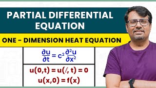
The heat conduction equation is framed for a semi-infinite rod, where one end is maintained at a constant temperature, leading to the application of the Fourier Cosine Transform. This process establishes a solution method to derive temperature distribution over time, using appropriate boundary and initial conditions.
Detailed
Application of Heat Equation in a Semi-Infinite Rod
This section delves into a particular application of the Fourier Cosine Transform in solving the heat equation for a semi-infinite rod, represented mathematically as follows:
- Governing Equation:
$$ \frac{\partial u}{\partial t} = \alpha^2 \frac{\partial^2 u}{\partial x^2}, \quad x>0, \; t>0 $$
Subject to the conditions:
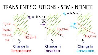
1. $$ u(0,t) = T $$ (end held at constant temperature)
2. $$ u(x,0) = 0 $$ (initial temperature is zero)
3. $$ \lim_{x \to \infty} u(x,t) = 0 $$ (temperature approaches zero far from the boundary)
By applying the Fourier Cosine Transform, which is suited for problems defined over a semi-infinite domain, we convert the partial differential equation into an ordinary differential equation. This can be solved by finding the function $U(s,t)$, leading to an exponential solution.
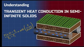
The final temperature distribution in the rod is expressed with the complementary error function:
$$ u(x,t) = T ext{erfc} \left( \frac{x}{2\sqrt{\alpha t}} \right) $$
This process illustrates the strength of Fourier Cosine Transforms in addressing boundary value problems, especially in engineering applications like thermal analysis.
Youtube Videos

Audio Book
Dive deep into the subject with an immersive audiobook experience.
Description of the Semi-Infinite Rod Problem
Chapter 1 of 7
🔒 Unlock Audio Chapter
Sign up and enroll to access the full audio experience
Chapter Content
Consider a semi-infinite rod x ∈ [0,∞) initially at zero temperature, and for t > 0, the end x = 0 is held at a constant temperature T.
Detailed Explanation
This chunk introduces the physical setup of the problem. We have a rod that stretches infinitely in the positive x-direction, where we initially assume the entire rod is at a temperature of zero. At some point, we start heating the very beginning of the rod (x = 0) to a temperature T, which will cause heat to travel along the rod over time. Understanding this setup is crucial as it establishes the conditions under which we will analyze heat conduction.
Examples & Analogies
Think of a long metal rod partially submerged in hot water, where only the end of the rod touching the water heats up. Over time, the heat transfers along the rod, illustrating similar principles to our semi-infinite rod problem.
Governing Equation of Heat Conduction
Chapter 2 of 7
🔒 Unlock Audio Chapter
Sign up and enroll to access the full audio experience
Chapter Content
The governing equation is the heat conduction equation:
∂u/∂t = α² ∂²u/∂x², x > 0, t > 0.
Detailed Explanation
This chunk presents the mathematical formulation describing how temperature changes over time (∂u/∂t) and how it changes along the rod (∂²u/∂x²). Here, u represents the temperature at a position x and time t, while α² is a constant that reflects the material properties of the rod. This equation is a partial differential equation (PDE) that enables us to model the physical process of heat conduction mathematically.
Examples & Analogies
Imagine turning on a hair straightener. The straightener gets hot, and that heat gradually moves through the metal plates. The equation describes how the temperature in the plate evolves both over time and from one end to the other.
Boundary and Initial Conditions
Chapter 3 of 7
🔒 Unlock Audio Chapter
Sign up and enroll to access the full audio experience
Chapter Content
Subject to:
- u(0,t) = T,
- u(x,0) = 0,
- lim (x→∞) u(x,t) = 0.
Detailed Explanation
Here, we define specific conditions that apply to our problem: At the boundary (x=0), the temperature is held constant at T. Initially (at time t=0), the entire rod is at zero temperature, and as we move infinitely far from the heated end, the temperature approaches zero. These conditions are critical as they define how we will solve our governing equation and find the temperature distribution over time.
Examples & Analogies
Think of holding one end of a thick blanket over a heater while the other end is outside in the cold. Initially, the entire blanket feels cold (zero temperature), but as you keep it near the heater, one end gets hot (temperature T), while far away (as you move along the blanket), the warmth fades back to coldness.
Solution Approach Using Fourier Cosine Transform
Chapter 4 of 7
🔒 Unlock Audio Chapter
Sign up and enroll to access the full audio experience
Chapter Content
We take the Fourier Cosine Transform with respect to x:
Let U(s,t)=F {u(x,t)}= (2/π) ∫₀^∞ u(x,t)cos(sx)dx.
Detailed Explanation
To solve the heat equation, we apply the Fourier Cosine Transform, which is useful for problems defined over semi-infinite domains. This transform helps convert the partial differential equation into an ordinary differential equation (ODE) in the time domain, simplifying the calculations. U(s,t) represents the transformed version of the temperature function u(x,t), and the integral computes how much of each cosine function contributes to the overall temperature distribution.
Examples & Analogies
Imagine using a prism to decompose light into different colors. In our case, the Fourier transform is like a prism that decomposes the temperature profile into simpler components, allowing easier analysis.
Deriving the ODE
Chapter 5 of 7
🔒 Unlock Audio Chapter
Sign up and enroll to access the full audio experience
Chapter Content
Using properties of derivatives under transforms:
F{ ∂²u/∂x²} = −s²U(s,t),
∂U/∂t = −α²s²U(s,t).
Detailed Explanation
This chunk provides the transition to an ordinary differential equation. The Fourier transform of the second spatial derivative introduces a term involving s² (the frequency variable), while the Fourier transform of the time derivative results in a straightforward time derivative. This leads to a first-order linear ordinary differential equation for U(s,t), which is easier to solve compared to the original PDE.
Examples & Analogies
Think of transforming a complex task into a series of easier steps. Just like how breaking down a complicated recipe into simple instructions makes cooking easier, transforming the temperature equation into an ODE simplifies finding the solution.
General Solution and Initial Condition
Chapter 6 of 7
🔒 Unlock Audio Chapter
Sign up and enroll to access the full audio experience
Chapter Content
This is a first-order linear ODE in t with solution:
U(s,t)=A(s)e^{−α²s²t}.
From initial condition u(x,0)=0 ⇒ U(s,0)=0 ⇒ A(s)=0, but this contradicts the boundary condition.
Detailed Explanation
We find that the solution for U(s,t) is of an exponential form, which is typical for heat equations. However, applying the initial condition directly leads to a contradiction regarding the constant A(s). This situation indicates that we cannot simply apply the initial condition without properly addressing the steady-state boundary condition at the same time.
Examples & Analogies
Consider starting a plant from a seed. If you plant an initial seed in 'zero' conditions (no water, no sun), while wanting it to grow immediately, it doesn't work. In our mathematical scenario, we need to find a suitable condition to connect initial feelings with final results.
Addressing the Non-Homogeneous Boundary Condition
Chapter 7 of 7
🔒 Unlock Audio Chapter
Sign up and enroll to access the full audio experience
Chapter Content
To fix this, we transform the non-homogeneous boundary via suitable substitution (e.g., Duhamel’s principle or separation of variables), which leads to:
u(x,t)=T erfc(√(x/(2αt))).
Detailed Explanation
To resolve the issues with the boundary conditions, we apply techniques like Duhamel's principle or separation of variables, which help us incorporate the effect of the constant temperature boundary condition and lead us to the final solution using the complementary error function. This solution provides temperature at any point of the rod over time with respect to the specified boundary conditions.
Examples & Analogies
It's like using special gardening techniques to ensure each plant (here, the solution) receives the right combination of conditions to thrive. We adapt our calculations to produce a result that respects both the initial and boundary conditions.
Key Concepts
-
Heat conduction involves transferring heat through a medium, and the heat equation governs this process.
-
The Fourier Cosine Transform is key in solving boundary value problems in semi-infinite domains.
-
Boundary conditions define how a system behaves at its limits, affecting the solutions derived from differential equations.
-
The complementary error function is useful in expressing solutions related to heat conduction.
Examples & Applications
A semi-infinite rod at constant temperature at one end demonstrates the use of Fourier transforms to study temperature changes over time.
By applying boundary conditions, we see how heat diffuses from the end of a rod into the surrounding material.
Memory Aids
Interactive tools to help you remember key concepts
Rhymes
Heat in a rod must not be odd, it flows to the cold, from the warm bestowed.
Stories
Imagine a stick in a warm fire, one end is red hot while the rest desires. As time goes on, the heat spreads wide, until the cold end can no longer hide.
Memory Tools
For the heat equation remember: A for alpha, T for temperature, x for position, t for time!
Acronyms
HEAT - Heat Equation Applied Theory in a semi-infinite rod.
Flash Cards
Glossary
- Semiinfinite Rod
A rod that extends infinitely in one direction and has a boundary at the other end.
- Heat Equation
A partial differential equation that describes how heat diffuses through a given region over time.
- Fourier Cosine Transform
An integral transform that converts a function defined on a semi-infinite interval into a frequency domain using cosine functions.
- Complementary Error Function (erfc)
A special function that quantifies the tails of a normal distribution, often used in calculations involving heat transfer.
Reference links
Supplementary resources to enhance your learning experience.