
Solving PDEs Using Fourier Sine Transform
Enroll to start learning
You’ve not yet enrolled in this course. Please enroll for free to listen to audio lessons, classroom podcasts and take practice test.
Interactive Audio Lesson
Listen to a student-teacher conversation explaining the topic in a relatable way.
Introduction to Wave Equation
🔒 Unlock Audio Lesson
Sign up and enroll to listen to this audio lesson

Today, we will dive into the wave equation, which serves as a foundational model for understanding wave propagation. It's given by the formula \( \frac{\partial^2 u}{\partial t^2} = c^2 \frac{\partial^2 u}{\partial x^2} \). Can anyone tell me what the variables \( u \) and \( c \) represent?

I think \( u \) represents the displacement of the wave, and \( c \) is the speed of the wave.
Exactly! The displacement describes how far a point in the medium moves from its rest position, while \( c \) is the speed at which waves travel through the medium. Remember, we will analyze this equation under specific boundary conditions.

What kind of boundary conditions are we discussing?
Great question! In this section, we consider conditions where the displacement vanishes at the boundary, specifically at \( x = 0 \). This is perfect for using the Fourier Sine Transform!
Applying the Fourier Sine Transform
🔒 Unlock Audio Lesson
Sign up and enroll to listen to this audio lesson

Now, with our wave equation and boundary conditions in place, we apply the Fourier Sine Transform. The transformation is given by \( U(s,t) = F \{ u(x,t) \} \). How do you think this changes our equation?

I suppose it changes it from a partial differential equation to an ordinary differential equation?
Exactly! It allows us to transform our PDE into an ODE with respect to \( t \) and we get \( \frac{\partial^2 U}{\partial t^2} = -c^2 s^2 U \). Let's think about what kind of solution forms we can derive from this ODE.

Are we looking for solutions like we do for normal differential equations?
Precisely! The solution to this type of ODE generally leads to terms involving sine and cosine, which makes sense given our wave context!
Integrating Back to the Original Function
🔒 Unlock Audio Lesson
Sign up and enroll to listen to this audio lesson
After solving the ODE, we arrive at the solution \( U(s,t) = A(s) \cos(cst) + B(s) \sin(cst) \). But remember, we had initial conditions that helped us determine some properties of our functions. What happened to \( B(s) \) in this case?
Since \( B(s) \) is related to the initial velocity, and because it was given that there was no external force acting at the start, it becomes zero.
Correct! So, we can simplify our expression to \( U(s,t) = A(s) \cos(cst) \). Afterwards, how do we convert back to our original domain?
We would need to apply the inverse Fourier Sine Transform!
Exactly! And this is how we express the solution to our physical problem, illustrating how the displacement evolves over time under the wave equation. Let's recap!
Importance of Fourier Sine Transform in Engineering
🔒 Unlock Audio Lesson
Sign up and enroll to listen to this audio lesson
Finally, let’s touch on the significance of using the Fourier Sine Transform in engineering applications. Can anyone share where they think it might be useful?
Maybe in analyzing vibrations in structures, like bridges?
Absolutely! It's essential for understanding anything that involves vibrations or wave propagation in engineering. Remember, any time you encounter a boundary condition that specifies zero displacement, you can consider using the Fourier Sine Transform.
It sounds really powerful! How does it relate to thermal problems?
That's a great connection! Many thermal conduction problems can be expressed similarly, using Fourier transforms to simplify the analysis.
Introduction & Overview
Read summaries of the section's main ideas at different levels of detail.
Quick Overview
Standard
The section discusses the Fourier Sine Transform's role in addressing PDEs with boundary conditions at x=0 where solutions vanish. The focus is on the wave equation, presenting the formulation, initial conditions, and the resulting solutions, along with an example that illustrates this process.
Detailed
Solving PDEs Using Fourier Sine Transform
Brief Overview
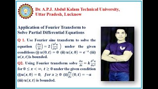
This section addresses the application of the Fourier Sine Transform (FST) in solving partial differential equations (PDEs) under specific boundary conditions, particularly where the solution is zero at the boundary (x=0). This is essential in various engineering problems dealing with vibrations and wave motion.
Key Points
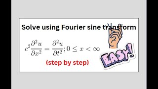
- Wave Equation Introduction: The one-dimensional wave equation is presented as \( \frac{\partial^2 u}{\partial t^2} = c^2 \frac{\partial^2 u}{\partial x^2} \), outlining the physical context where it applies.
- Boundary Conditions: The problem requires setting well-defined boundary conditions to exploit the properties of the FST. Here, \( u(0,t) = 0 \), and the limits as \( x \to \infty \) state that the wave diminishes.
- Application of Fourier Sine Transform: The Fourier Sine Transform is applied to transform the spatial domain (x) into the frequency domain (s), resulting in a second-order ordinary differential equation (ODE) in time (t).
- Solution Formulation: By solving the resultant ODE, it is found that the solution takes the form \( U(s,t) = A(s) \cos(cst) + B(s) \sin(cst) \), with initial conditions leading to \( B(s) = 0 \).
- Final Integral Solution: The displacement of the vibrating rod is expressed through an integral involving the Fourier Sine Transform of the initial displacement function, giving insight into how to derive the time-evolved solution from the initial conditions and transformed function.
Importance
This method is significant in understanding vibrations and wave propagation in structural components, showcasing the Fourier Sine Transform's utility in engineering contexts.
Youtube Videos


Audio Book
Dive deep into the subject with an immersive audiobook experience.
Overview of PDEs with Boundary Conditions
Chapter 1 of 4
🔒 Unlock Audio Chapter
Sign up and enroll to access the full audio experience
Chapter Content
Now consider problems where the solution vanishes at the boundary x = 0, which is ideal for Fourier Sine Transform.
Detailed Explanation
This chunk introduces the context where Fourier Sine Transform (FST) is effectively applied. In many physical situations, especially in mechanical and civil engineering, we encounter problems where a function approaches zero at the boundary (here, at x = 0). This feature of vanishing conditions at the boundaries makes Fourier Sine Transform the appropriate tool, as it is specifically designed to handle such cases. Thus, if we expect our solution to decay to zero at the boundaries, we would opt for FST over other transforms.
Examples & Analogies
Imagine holding one end of a rope tightly (this represents the boundary at x = 0) while the other end dangles freely. The vibrations or movements you create start at the fixed end but gradually diminish as they travel along the rope towards the free end. In this scenario, the Fourier Sine Transform effectively models how the vibrations are controlled from the boundary condition to the end of the rope, where they eventually disappear.
Wave Equation Analysis
Chapter 2 of 4
🔒 Unlock Audio Chapter
Sign up and enroll to access the full audio experience
Chapter Content
Let us consider the one-dimensional wave equation:
∂²u/∂t² = c² ∂²u/∂x²
With boundary conditions:
u(0,t)=0,
lim (x→∞) u(x,t)=0,
u(x,0)=f(x),
∂u/∂t |_(t=0)=0
Detailed Explanation
In this chunk, we are presented with the one-dimensional wave equation, which describes how wave-like phenomena propagate through a medium. The equation itself includes second derivatives with respect to both time (t) and space (x), meaning it captures the acceleration of wave displacement over time and the spatial characteristics of the wave. The boundary conditions specify that at the fixed location x = 0, the displacement must always be zero, and as we move further away (toward infinity), the displacement should approach zero. The initial conditions outline that we've started with an initial shape of the wave defined by f(x) and that the initial velocity of the wave is zero.
Examples & Analogies
Think of a stretched membrane, like a drum skin, where striking the drum creates waves that ripple outwards. The point where you strike (where the drum is fixed) represents the boundary condition (u(0,t) = 0), where there's no displacement of the membrane at the rim, while the waves themselves diminish as they travel further from the source, consistent with the condition that the wave height approaches zero at infinity.
Applying the Fourier Sine Transform
Chapter 3 of 4
🔒 Unlock Audio Chapter
Sign up and enroll to access the full audio experience
Chapter Content
Apply the Fourier Sine Transform:
∂²U/∂t² = -c²s²U
This is a second-order ODE in t:
U(s,t)=A(s)cos(cst)+B(s)sin(cst)
Detailed Explanation
Once we apply the Fourier Sine Transform to the wave equation, we end up with a transformed equation that represents the same physical phenomenon in the frequency domain. This transformed equation is a second-order ordinary differential equation (ODE) in terms of time t. The general solution to this ODE is expressed in terms of sine and cosine functions, where A(s) and B(s) are coefficients that depend on the transformed initial conditions. The cosine term represents the oscillations of the wave associated with the initial shape, while the sine term would account for any initial velocities.
Examples & Analogies
Returning to our drum example, if one were to tap the drum softly, it would create a sound wave characterized by specific frequencies (higher and lower notes). The sine and cosine functions represent these frequencies, capturing the essence of how the drum vibrates over time, thus allowing us to predict how the sound changes shortly after you hit it based on the initial conditions.
Obtaining Displacement Solution
Chapter 4 of 4
🔒 Unlock Audio Chapter
Sign up and enroll to access the full audio experience
Chapter Content
Initial conditions give:
U(s,0)=F{s{f(x)}}=A(s), ∂U/∂t|_(t=0)=0⇒B(s)=0
Thus,
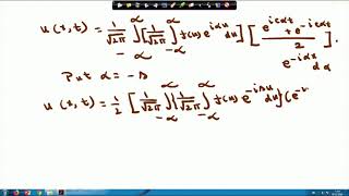
U(s,t)=F{f(x)}·cos(cst)
⇒u(x,t)=F{f(x)}cos(cst)sin(sx)ds
Detailed Explanation
This chunk illustrates how the coefficients obtained from the initial conditions help refine our solution for U(s,t). In this case, since the initial velocity of the wave is set to zero, it simplifies the solution by eliminating the B(s) term. Thus, the solution U(s,t) depends solely on the initial shape of the wave and oscillates with cosine over time. We then perform the inverse transform to get the actual displacement function u(x,t) in terms of the original function f(x) and sine terms, encapsulating how the wave travels through the medium over time.
Examples & Analogies
Imagine being at a concert. The musicians start playing a familiar tune (f(x) is the orchestra’s performance). Half a second in, there's absolute silence at the start (initial velocity is zero), resulting in a smooth wave pattern of sound traveling outwards to the audience. The final displacement function reflects both the initial tune played and the nature of how sound waves propagate through the air (represented by the sine terms, affecting where the sound is heard over time).
Key Concepts
-
Wave Equation: A fundamental equation in physics showing the relationship between time and spatial changes in wave propagation.
-
Boundary Conditions: Essential constraints needed to solve PDEs accurately in specific contexts.
-
Fourier Sine Transform: A specific type of Fourier transform effective for functions defined on semi-infinite domains.
Examples & Applications
Using the Fourier Sine Transform to solve the wave equation for a vibrating rod with one end fixed at zero displacement, leading to the integral solution involving the Fourier sine transform of the initial function.
Memory Aids
Interactive tools to help you remember key concepts
Rhymes
When waves do start to sway, their displacement we'll convey, with Sine Transform in play, equations find their way.
Stories
Imagine a massive bridge swaying with the wind; it must not collapse. Now, with boundary conditions set, we apply the Fourier Sine Transform to ensure its safe vibrancy, crafting solutions that give peace of mind to engineers.
Memory Tools
F-Sine for 'Free Low': 'F' for Fourier, 'Sine' for function vanishing at one end, indicates applying Fourier Sine Transform.
Acronyms
BVS
Boundary Value Solutions using Fourier Sine.
Flash Cards
Glossary
- Fourier Sine Transform (FST)
A mathematical transform that converts a function defined on a semi-infinite domain into a series of sine functions.
- Wave Equation
A second-order linear partial differential equation that describes how wave functions propagate over time.
- Boundary Condition
Conditions that specify the behavior of a function at the boundaries of its domain.
- Integral Solution
The solution to a differential equation expressed as an integral.
Reference links
Supplementary resources to enhance your learning experience.