
Finite Difference Method (FDM)
Enroll to start learning
You’ve not yet enrolled in this course. Please enroll for free to listen to audio lessons, classroom podcasts and take practice test.
Interactive Audio Lesson
Listen to a student-teacher conversation explaining the topic in a relatable way.
Introduction to Finite Difference Method
🔒 Unlock Audio Lesson
Sign up and enroll to listen to this audio lesson

Today, we are going to discuss the Finite Difference Method or FDM, which is a numerical approach for approximating solutions to differential equations, particularly the two-dimensional wave equation. Have any of you heard of FDM before?

I think I have. It's about using grids to solve equations, right?
Exactly! FDM involves discretizing the domain into a grid. Each grid point corresponds to a specific value of the function we are analyzing. Why do you think this grid approach is helpful?

I guess it makes complex problems simpler by breaking them into smaller parts?
That's right! By splitting the problem into smaller, manageable pieces, we can compute values systematically. Remember, FDM is particularly useful when analytical solutions are hard to come by.
Discretization and Grid Structure
🔒 Unlock Audio Lesson
Sign up and enroll to listen to this audio lesson

Now, let's talk about how we actually set up our grid. We need to define our spatial step sizes, Δx and Δy, as well as our time step Δt. Can someone explain why these parameters are important?

They determine the resolution of our grid, right? Smaller steps mean a more accurate solution?
Yes! However, there are trade-offs. While smaller step sizes increase accuracy, they also require more computational power. We have to balance resolution and computational efficiency.

So, how do we apply these step sizes in calculations?
Good question! Each grid point’s displacement is represented as un_i,j for the point at coordinates (i,j) and time level n.
Explicit Finite Difference Scheme
🔒 Unlock Audio Lesson
Sign up and enroll to listen to this audio lesson
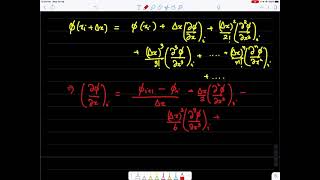
Let's delve into the explicit finite difference scheme. The formula we use to compute the displacement at the next time level, un+1_i,j, is quite comprehensive. It includes contributions from the past time levels and neighboring grid points. Can anyone restate what the general form of that equation looks like?
It goes something like un+1 equals two times un minus un-1, plus some terms involving the neighboring points, right?
Exactly! This relationship is the heart of FDM. It allows us to evolve the solution over time based on previous values.
What do those neighboring points do in the equation?
Great question! They provide a broader context for calculating the new displacement by considering how the dynamics at those points influence the value at our focused point.
Stability Condition (CFL Condition)
🔒 Unlock Audio Lesson
Sign up and enroll to listen to this audio lesson
Lastly, let's discuss the stability condition known as the CFL condition, which is vital for ensuring our numerical solution remains stable over time. Can anyone explain what this condition entails?
It’s something about keeping the ratios of step sizes in check, right? Like ensuring a certain value doesn't exceed a limit?
Exactly! The CFL condition states that (cΔt)²/Δx² + (cΔt)²/Δy² must be less than or equal to 1. This prevents numerical oscillations from growing out of control. Keeping stability ensures our computations are valid.
What happens if we exceed that limit?
Good question! Exceeding that limit can lead to unstable solutions, making the results unreliable. Therefore, it’s crucial to always check your parameters. Does anyone have any questions about today's topic?
Introduction & Overview
Read summaries of the section's main ideas at different levels of detail.
Quick Overview
Standard
In this section, the Finite Difference Method (FDM) is discussed as a numerical technique to approximate solutions to the 2D wave equation. By discretizing the domain into a grid and establishing an explicit scheme, it allows for solving complex scenarios where analytical solutions are impractical, while also emphasizing the importance of stability conditions to ensure the accuracy of solutions.
Detailed
Finite Difference Method (FDM)
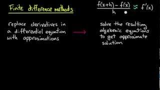
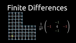
The Finite Difference Method (FDM) is a critical numerical technique used for solving differential equations, especially in scenarios where analytical solutions are insufficient or impractical. This method is particularly valuable in civil engineering applications involving the two-dimensional wave equation governing vibrating membranes. The basic premise of the FDM involves discretizing the spatial and temporal domain into a grid, which allows for the approximation of derivatives through finite differences.
Discretization and Grid Structure
- The domain is divided into a grid defined by step sizes Δx and Δy in space, and Δt in time.
- The approximation for the displacement at any grid point (i,j) at time level n is denoted by un_i,j.
Explicit Finite Difference Scheme
- The explicit scheme for the 2D wave equation is formulated as:
un+1_i,j = 2un_i,j - un-1_i,j + (cΔt)²
  (un_i+1,j - 2un_i,j + un_i-1,j)/(Δx)² + (cΔt)²
  (un_i,j+1 - 2un_i,j + un_i,j-1)/(Δy)²
- Here, the new value of displacement at time n+1 is expressed in terms of past values and involves contributions from neighboring grid points.
Stability Condition (CFL Condition)
- A key aspect of using FDM is ensuring computational stability, typically governed by the Courant-Friedrichs-Lewy (CFL) condition:
(cΔt)²/Δx² + (cΔt)²/Δy² ≤ 1
- This condition ensures that numerical oscillations do not grow uncontrollably, thereby making the solution stable over time. Understanding and applying the CFL condition is essential for successful numerical simulation of wave phenomena.
Youtube Videos


Audio Book
Dive deep into the subject with an immersive audiobook experience.
Discretizing the Domain
Chapter 1 of 3
🔒 Unlock Audio Chapter
Sign up and enroll to access the full audio experience
Chapter Content
Discretize the domain into a grid:
Let:
- un be the approximation of u(x , y ,t ),
- Δx, Δy: spatial step sizes,
- Δt: time step.
Detailed Explanation
To apply the Finite Difference Method (FDM), we begin by discretizing the continuous domain of the membrane into a grid. This means we break down the area we want to analyze into a set of discrete points or nodes where we will perform our calculations. Here, 'un' represents the approximation of the membrane displacement at point (i,j) at time 'n'. The parameters Δx and Δy denote the spacing or step sizes between these grid points in the spatial dimensions, while Δt is the time step we take between each calculation in time.
Examples & Analogies
Imagine you are trying to measure the temperature on a large square field. Instead of taking one measurement for the entire area, you set up a grid and take measurements at equally spaced points. This way, you can get a detailed understanding of how temperature varies across the field, just as we do with the membrane surface using FDM.
Explicit Finite Difference Scheme
Chapter 2 of 3
🔒 Unlock Audio Chapter
Sign up and enroll to access the full audio experience
Chapter Content
The explicit finite difference scheme for the 2D wave equation is:
un+1 = 2un − un−1 + (cΔt)²
((un − 2un + un)
+ (cΔt)² (un − 2un + un)
)
Detailed Explanation
Using the finite difference method, we can find the displacement of the system at the next time step (n+1) based on past displacements at the current time step (n) and the previous time step (n-1). The equation combines the contributions from previous time steps and incorporates the wave speed 'c' and the spatial step sizes Δx and Δy, allowing us to calculate how the membrane behaves over time. The two terms involving the double differences reflect the influence of neighboring points in the grid.
Examples & Analogies
Think of it like predicting the future movements of people in a crowd. If we know where people are standing now and where they were standing a moment ago, we can make an educated guess about where they will be next, factoring in their speed – this is similar to how we calculate future positions of points on the membrane.
Stability Criterion (CFL Condition)
Chapter 3 of 3
🔒 Unlock Audio Chapter
Sign up and enroll to access the full audio experience
Chapter Content
Stability Criterion (CFL condition):
(cΔt)² + (cΔt)² ≤ 1
Δx Δy
This ensures that the solution remains stable over time.
Detailed Explanation
The stability of the numerical solution is crucial for obtaining accurate results. The Courant-Friedrichs-Lewy (CFL) condition helps us determine a safe choice for the time step (Δt) relative to the spatial steps (Δx and Δy) and the wave speed (c). This condition essentially states that if the value we choose for the time step is too large in relation to the spatial steps, our calculations may become unstable, leading to nonsensical results. Adhering to this condition helps ensure that our simulation remains valid and progresses accurately.
Examples & Analogies
Consider riding a bicycle on a winding path. If you try to pedal too fast (large Δt) while navigating tight turns (small Δx and Δy), you risk losing control and falling over. Similarly, the CFL condition helps us maintain control over our simulations to ensure smooth and reliable outputs.
Key Concepts
-
Discretization: Refers to breaking down the domain into a grid format with specific step sizes.
-
Explicit Scheme: A numerical method that calculates future values from current and past data directly.
-
Stability Condition: A criterion that ensures the numerical solution remains valid over time.
Examples & Applications
Using grid sizes of Δx = Δy = 0.1 m and Δt = 0.01 s, compute the displacement at a point in a vibrating membrane over several time steps.
In a structure modeled by the 2D wave equation, apply FDM to analyze how varying the step size affects the accuracy of the solution.
Memory Aids
Interactive tools to help you remember key concepts
Rhymes
Finite Differences keep us on track, / With grids to give our answers back!
Stories
Imagine a group of travelers mapping out a grand adventure through unknown terrain. They divided the land into sections, exploring one at a time, just as FDM breaks down complex equations into manageable grid pieces.
Memory Tools
Remember 'Gains Stability': Grid, Approximation, Iteration, Numerical, Stability, Time step. This can help recall steps supported by FDM.
Acronyms
FDM = Fast Discrete Mapping! Think of numerically mapping out wave equations swiftly with a structured grid.
Flash Cards
Glossary
- Finite Difference Method (FDM)
A numerical approach for approximating solutions to differential equations by discretizing the spatial and temporal domain into a grid.
- Discretization
The process of dividing a continuous function into discrete points for analysis.
- Explicit Finite Difference Scheme
A method where future values are computed directly from known current and past values at grid points.
- CFL Condition
A stability criterion providing conditions under which a numerical method for solving partial differential equations will yield stable solutions.
Reference links
Supplementary resources to enhance your learning experience.